Measurement Scale and Upper Tail Sensitivity in Positive Data Model Comparison

1Introduction

Positive-data models are often selected from a table of information criteria and goodness-of-fit statistics. Such a table shows how the specified models compare on the observed sample. Choosing a model for a high quantile also requires scrutiny of its tail, the likelihood solution and the units used in fitting. These concerns become particularly acute when only a small sample is available.

Exponential, Weibull, gamma and Fréchet distributions provide familiar reference models. Burr–Hatke constructions offer a wider range of density and hazard shapes. Yadav et al. [1] studied the scaled Burr–Hatke exponential model. Afify et al. [2] introduced an inverse-power construction, Abubakari et al. [3] applied a Chen generating map, and Anyiam et al. [4] developed a Topp–Leone extension. Their different constructions also warrant a closer examination of how each model behaves when the measurement units change.

Penalized likelihood criteria balance agreement with the sample against the number of fitted parameters. Akaike’s criterion targets a predictive trade-off, while the Bayesian information criterion uses a different complexity penalty [5], [6]. A small-sample correction is useful when the sample is small relative to the parameter count [7], [8]. Leave-one-out log scoring assesses each observation using a model fitted without that observation [9]. Agreement between these summaries helps interpretation, but their differences can also reveal which aspect of fit drives a ranking.

Upper-tail prediction raises a further difficulty. Two fitted distribution functions can agree closely over the observed range and give quite different quantiles beyond it. A polynomial tail and an exponentially damped tail make different extrapolations. A few large observations may favour the heavier tail even when the aggregate predictive score favours a lighter-tailed model. We therefore examine upper quantiles alongside the overall model comparison.

Measurement units matter when the model contains a fixed numerical reference. A scale family fitted in one unit has an equivalent representation in another: its fitted probabilities are unchanged, and its density acquires the usual Jacobian factor. A family with a fixed reference need not have this property. Applying its raw formula after changing units can therefore change the family being fitted. The resulting change in fit needs to be interpreted through the model specification.

We investigate these issues through eight established distributions and three published observation vectors. The main analytical results concern the median constraint and lack of scale closure of the unscaled IPBH family. The empirical analysis examines their consequences, checks a retained likelihood solution and calculates new leave-one-out scores and upper-quantile sensitivities. All fits reported here were calculated afresh from the vectors in Appendix B. Section II describes the models, derivations and assessment methods; Section III presents the results. Sections IV and V discuss their implications and conclusions.

2Methods

2.1Candidate distributions

2.1.1Definitions and parameter conventions

Table 1 summarizes the candidates. Every candidate has support $x>0$, with all parameters positive and location fixed at zero. We retain $\gamma$ for the inverse-scale parameter of BHE, TL-BHE and CBHE, $\alpha$ and $\beta$ for IPBH, and $\nu ,\xi ,\gamma$ for CBHE. For the classical shape and scale families we write $\kappa$ and $\sigma$. The number of fitted parameters is denoted by $k$ and must not be confused with $\kappa$.

Model	Parameters	k	Upper tail and scale structure
BHE	$\gamma$	1	Exponential damping with a scale parameter
TL-BHE	$\alpha ,\gamma$	2	Exponential damping with a scale parameter
CBHE	$\nu ,\xi ,\gamma$	3	Exponential damping with a scale parameter
IPBH	$\alpha ,\beta$	2	Polynomial decay with a fixed reference scale
Fréchet	$\kappa ,\sigma$	2	Polynomial decay with a scale parameter
Weibull	$\kappa ,\sigma$	2	Weibull decay with a scale parameter
Gamma	$\kappa ,\sigma$	2	Exponential damping with a scale parameter
Exponential	$\lambda$	1	Exponential decay with a scale parameter

2.1.2Burr–Hatke exponential models

The scaled BHE baseline is written as $G=1-s$, where

The BHE distribution has $F_{\mathrm{BHE}}=G$ and $f_{\mathrm{BHE}}=g$. Its hazard is $\gamma (2+\gamma x)/(1+\gamma x)$, decreasing from $2\gamma$ to $\gamma$. Its dependence on $\gamma x$ makes its scale structure explicit. The Topp–Leone transformation gives [4]

For CBHE, define $v=G^{\xi }$, $E=e^v-1$ and $d_{\nu }=1-e^{-\nu (e-1)}$. The normalized Chen map gives [3]

The denominator in this expression is part of the model definition. Since $G$ tends to one, $E$ tends to $e-1$; division by $d_{\nu }$ ensures that the CDF tends to one. Both generating maps are increasing, and differentiating them gives the stated densities. They therefore preserve positivity and normalization without requiring an infinite density expansion.

2.1.3Inverse power Burr–Hatke model

The IPBH form of Afify et al. [2], with the second shape parameter denoted here by $\beta$, is

Put $u=x^{-\beta }$ and $h=\alpha +{(1+u)}^{-1}$. Differentiation using $du/dx=-\beta u/x$ yields

The constant one in the denominator is a fixed reference. It cannot be replaced by $\alpha$ or absorbed into $\alpha$ through a change of units. This differs from a model depending only on a fitted product such as $\gamma x.$ Section II.B develops the consequences directly from the CDF.

2.1.4Classical comparison models

The exponential distribution has $F\left(x\right)=1-e^{-\lambda x}$ and $f\left(x\right)=\lambda e^{-\lambda x}$. For Weibull,

The gamma density and CDF are

Here $P(\kappa ,z)$ denotes the regularized lower incomplete gamma function. These are the zero-location parameterizations in the NIST/SEMATECH handbook [10]. The Fréchet candidate is

The classical models separate shape from scale. In particular, changing $\sigma$ translates the quantile curve proportionally. The comparison therefore includes two one-parameter models, five two-parameter models and one three-parameter model. Additional location parameters are not estimated.

2.1.5Tail behaviour relevant to extrapolation

For small positive $t$, $1-e^{-t}\sim t$. Applying this expansion to IPBH and Fréchet gives

Both tails decay as powers. Their positive $r$th moments exist only when $r<\beta$ and $r<\kappa$, respectively. This follows by integrating $r{x}^{r-1}S\left(x\right)$ at infinity. By comparison, $S_{\mathrm{BHE}}=s$ and

The TL-BHE expansion follows from $1-{(1-s^2)}^{\alpha }\sim \alpha s^2$. For CBHE, $G^{\xi }=1-\xi s+o\left(s\right)$, so $E=(e-1)-e\xi s+o\left(s\right);$ substitution into its normalized CDF gives the second result. These steps establish exponential damping for these two extensions. Weibull has survival $e^{-{(x/\sigma )}^{\kappa }}$ and gamma has an exponentially damped tail. All positive moments of these five candidates and the exponential candidate exist. For $\kappa <1$, the Weibull tail is stretched exponential; it is not polynomial.

2.2Measurement scale and model equivalence

2.2.1What a unit conversion should preserve

Let $Y=aX$, with a fixed conversion factor $a>0$. If a candidate family admits a parameter transformation $T_a$, the corresponding distribution and density satisfy

For BHE, TL-BHE and CBHE, $\gamma$ changes to $\gamma /a$ while the shape parameters remain fixed. For Weibull, gamma and Fréchet, $\sigma$ changes to $a\sigma$; for exponential, $\lambda$ changes to $\lambda /a$. The fitted probabilities and all empirical-CDF discrepancies are therefore identical. Summing the density relation over a sample gives

The same additive term affects all equivalent candidate likelihoods. Thus an absolute AICc value changes with units, while its differences and ranking do not. Subtracting $2n\log a$ from a rescaled AICc places it on the original scale. A density comparison that ignores this adjustment can mistake a Jacobian effect for a change in fit.

2.2.2A fixed median constraint in the unscaled IPBH family

Proposition 1. For every $\alpha ,\beta >0$ in the unscaled IPBH family, its median exceeds one. If every observation is below one, its Kolmogorov–Smirnov distance exceeds one half.

Proof. Evaluation at one gives

Since the CDF is strictly increasing, its 0.5 quantile must lie above one. If $x_{\left(n\right)}<1$, the empirical CDF is one at $x_{\left(n\right)}$, but the fitted CDF remains below one half. Consequently,

This bound applies before estimation. The poor fit of an IPBH candidate to a sample entirely below one cannot be resolved by choosing different positive shape parameters. The restriction concerns the numerical reference used in the unscaled formula. It does not imply that all inverse-power constructions are unsuitable for small physical measurements.

2.2.3Lack of closure under rescaling

Proposition 2. A nontrivial linear rescaling of an unscaled IPBH variable cannot be represented by another member of the same two-parameter unscaled family.

Proof. If $X$ has the IPBH CDF, then $Y=aX$ has

Suppose this CDF equals $\exp (-{\alpha }^{\star }{y}^{-{\beta }^{\star }})/(1+y^{-{\beta }^{\star }})$. As $y\downarrow 0$, its leading negative log-CDF term identifies ${\beta }^{\star }=\beta$ and ${\alpha }^{\star }=\alpha a^{\beta }$. As $y\to \infty$, the leading survival coefficient of the transformed CDF is $(\alpha +1)a^{\beta }$. Equality with the candidate coefficient ${\alpha }^{\star }+1$ then requires

Because $\beta >0$, this implies $a=1$. Hence a genuine unit change cannot be absorbed into the two shape parameters. This proof also explains why changing only the coefficient in the exponential part is insufficient: the denominator carries a second scale dependence.

2.2.4Declaring a physical reference scale

A measurement with physical units can first be expressed relative to a declared reference $c>0$ having the same units as $x$. Writing the original IPBH law for $x/c$ gives

Under a unit conversion, both $x$ and $c$ become $ax$ and $ac$, leaving the ratio unchanged. If $c$ is fixed externally before fitting, the number of estimated parameters remains two. If $c$ is estimated, it adds a parameter and defines a different candidate for model selection. Selecting $c$ after inspecting the fit also introduces adaptation that should be acknowledged. The rescaling experiment below audits the unscaled formula with its numerical reference held at one; it does not choose a favourable unit as an additional estimation step.

2.2.5Why IPBH can closely resemble Fréchet

The denominator term is negligible when $x^{-\beta }$ is small throughout the fitted range. More formally, put $\sigma ={\alpha }^{1/\beta }$ and evaluate the CDF at $x=\sigma z$. Then

This is the standardized Fréchet CDF. The limit does not make the finite-parameter families identical. It does explain why two separately listed candidates can make virtually the same fitted predictions in a particular sample. Near duplication affects the allocation of Akaike weights because those weights are normalized over the supplied candidate list.

2.3Maximum likelihood estimation and quantiles

2.3.1Common fitting principle

For observations $x_1,\dots ,x_n$, each candidate maximizes

The likelihood sums retain all observations, including repeated recorded values. The following reductions make the calculation simpler and more auditable than a generic multidimensional search for every candidate. All likelihoods are evaluated using the original positive observation vectors. Median standardization is used only when it preserves the candidate family through its explicit scale parameter.

2.3.2Exponential, gamma, Weibull and Fréchet estimators

The exponential estimate is $\widehat{\lambda }=1/\bar{x}$. For gamma, profiling its scale gives $\widehat{\sigma }=\bar{x}/\widehat{\kappa }$, where the shape solves

This follows by differentiating the gamma log likelihood first with respect to $\sigma$, substituting its solution, and then differentiating with respect to $\kappa$. Here $\psi$ is the digamma function. For Weibull, the conditional scale and shape equation are

For Fréchet, the analogous expressions use inverse powers:

Weighted sums in these equations are evaluated by subtracting the largest logarithmic term before exponentiation. This avoids overflow when powers are large. Each shape is obtained by a bracketed root calculation and its scale is then recovered from the corresponding profile formula.

2.3.3BHE and TL-BHE profile likelihoods

For BHE define $z_i=\gamma x_i$. Its rate score is

The contribution of each observation to its second derivative is

The score tends to positive infinity as $\gamma \downarrow 0$ and to $-\sum x_i$ as $\gamma \to \infty$. The log likelihood is strictly concave, so its rate solution is unique. For TL-BHE put $H_i=1-s_i^2$. Differentiation with respect to $\alpha$ yields the conditional estimate

We substitute this expression into the TL-BHE log likelihood and maximize the resulting one-dimensional function in $\log \gamma$. This is an exact profile reduction, not an approximation. A grid brackets the best profile region before bounded refinement. The original pair is subsequently checked in the full density.

2.3.4IPBH conditional maximization

For IPBH, with $u_i=x_i^{-\beta }$ and $h_i=\alpha +{(1+u_i)}^{-1}$, the log likelihood is

At fixed $\beta$, the first two derivatives in $\alpha$ are

At $\alpha =0$ the score equals $n$, because $h_i^{-1}=1+u_i$. Its limit as $\alpha \to \infty$ is $-\sum u_i$. Hence the conditional estimate is unique and positive. The bound $\alpha =2n/\sum u_i$ gives a negative score and supplies a finite upper root bracket. We solve this scalar equation for each trial $\beta$ and maximize the profile over $\log \beta$.

This calculation has a practical advantage. It cannot retain an inferior value of the first parameter merely because a two-dimensional optimizer stops along a shallow region. The profile grid spans log shape values from −7 to 3.5, with 45 equally spaced points, followed by bounded refinement around its best point. The fitted profile solutions in the present datasets are well inside this search range. The reported source solution is also evaluated explicitly as a numerical benchmark in Section III.

2.3.5CBHE search and numerical checks

CBHE requires a joint search. With $L_i=\log G_i$, $v_i=G_i^{\xi }$ and $E_i=e^{v_i}-1$, its log likelihood is

Analytical gradients are given in Appendix A. Full-sample fits use 21 starting pairs formed from seven values of the first shape and three multiples of a TL-BHE shape estimate. The rate starts at twice the fitted TL-BHE rate on the standardized scale. A bounded quasi-Newton search is followed by simplex refinement and a final gradient calculation. Leave-one-out fits start from the full-sample estimate and three additional first-shape values. A wider search is used if convergence fails.

The full-sample fits and all leave-one-out fits satisfy the numerical checks, with no boundary solutions. This is evidence of stable numerical maximization under the specified protocol; it is not a proof that an arbitrary three-parameter likelihood has one global maximum. The density integrals, CDF derivatives and quantile inversions are checked independently for all eight candidates. Section III.G also verifies that the seven scale families retain their fitted likelihoods after an explicit unit conversion.

2.3.6Quantile calculation

For BHE, solving $s(x;\gamma )=1-p$ with $t=1+\gamma x$ gives $t{e}^t=e/(1-p)$. Thus

Here $W_0$ is the principal Lambert function [11]. For TL-BHE use the baseline probability $q=1-\sqrt{1-p^{1/\alpha }}$ in this inverse. For CBHE solve its generating map first:

For IPBH, the positive root of $\alpha u+\log (1+u)=-\log p$ gives $Q_{\mathrm{I}}\left(p\right)=u^{-1/\beta }$. This monotone root representation avoids subtracting nearly equal large Lambert-function values. The classical quantiles are

Gamma quantiles use $\sigma P^{-1}(\kappa ,p)$, and exponential quantiles use $-\log (1-p)/\lambda$. Every inversion is checked by substituting it back into the CDF. This is particularly useful when the upper quantile lies far beyond the largest observation.

2.4Data and assessment methods

2.4.1Observation vectors and source provenance

The mechanical sample contains 24 component failure times reproduced by Mandouh and Mohamed [12] from Murthy et al. [13]. The petroleum sample contains 48 positive measurements reproduced in DataSetsUni and ZeinEldin et al. [14]. The precipitation vector contains 100 annual maxima for Fort Collins, Colorado, over 1900–1999, as documented in DataSetsUni [15]. The observation vectors are reproduced in Appendix B, and Table 2 summarizes them. They retain the values used in the earlier thesis analysis.

The petroleum vector has one repeated value and the precipitation vector has 22 entries beyond its 78 distinct values. All entries are retained. Continuous densities are fitted to these recorded values; an interval likelihood would require a verified recording rule. The present observations do not identify those intervals, so the analysis does not introduce unverified jitter or rescaling constants. Quantiles are reported on the recorded numerical scales.

The examples were selected after model screening in the source study. They should therefore be treated as illustrative case studies rather than independent validation samples. Re-estimating parameters after leaving out one observation prevents that observation from entering its own fit, but it does not undo the earlier choice of datasets or candidate families. The precipitation calculations assess a marginal distribution under an exchangeable working sample; they are not chronological forecasting experiments.

Sample	n	Minimum	Median	Mean	Maximum	SD	Skewness
Mechanical	24	10.240000	19.240000	22.972500	51.560000	10.755022	1.437
Petroleum	48	0.090330	0.198862	0.218110	0.464125	0.083496	1.207
Precipitation	100	60.000000	158.000000	175.670000	463.000000	83.166871	1.357

All three vectors have positive sample skewness. The mechanical mean exceeds its median by about 3.73, and the petroleum and precipitation means also exceed their medians. These summaries describe asymmetric observed samples, but they do not by themselves identify a polynomial tail. Positive skewness and positive sample excess kurtosis are compatible with several of the light-tailed candidates as well.

2.4.2Information criteria and conditional weights

For each model with $k$ fitted parameters and maximized log likelihood $\widehat{\mathrm{l}}$, define

We use the conventional AICc expression as a common small-sample comparison rule, not as an exact finite-sample bias correction for every nonlinear candidate. BIC is also reported, while leave-one-out scores directly assess the fitted predictive density. These different summaries should not be counted as independent votes for a model.

Within each dataset, let ${\Delta }_m={\mathrm{AICc}}_m-{\min }_j{\mathrm{AICc}}_j.$ The normalized Akaike weight is

Weights summarize relative support conditional on the candidate list. They are not posterior probabilities that a distribution is literally true. They can change when a nearly duplicate candidate is added, even when its fitted predictions contribute little new information. We therefore report both the criterion differences and the weights.

2.4.3Empirical distribution discrepancies

For ordered observations, write $F_i=F(x_{\left(i\right)};\widehat{\theta })$. We calculate

The three measures summarize different aspects of fitted CDF agreement. Anderson–Darling assigns more weight to tail probabilities than the unweighted integrated discrepancy [16]. The values are descriptive fitted statistics. Standard fixed-distribution KS p-values are not supplied because parameters have been estimated from the same sample; the NIST/SEMATECH handbook [10] identifies simulation calibration as necessary in this situation. Ties and source selection would also need to be considered in a formal testing design.

2.4.4Exact leave-one-out log scores

For each observation, refit a candidate using the other $n-1$ entries. With this fitted vector denoted by ${\widehat{\theta }}_{m,-i}$, define

A larger score indicates a larger aggregate density assigned to held-out observations. Each model undergoes 172 held-out evaluations across the three samples. Identical held-out values have identical training vectors, so the 1,376 evaluations require 1,192 distinct fitting problems. Duplicate entries contribute separately to the final score. All fitting problems are checked, and none is dropped.

The log score is a density score, so its absolute value depends on measurement units. For an equivalent scale transformation, every held-out log density loses the same logarithm of the conversion factor. Consequently, ELPD changes by the same additive constant for all scale-equivalent candidates, and pairwise differences are preserved. We use the summed score rather than turning it into a claim of statistically significant superiority. The scores estimate marginal predictive performance within the observed sample setting.

2.4.5Tail and unit sensitivity summaries

The principal tail summaries are $Q\left(0.95\right)$ and $Q\left(0.99\right)$. To show how near-leading models differ, define a descriptive candidate set ${\mathrm{M}}_c=\{m:{\Delta }_m\le c\}$ and its quantile ratio

We evaluate $c=2,4,6$, retaining the threshold dependence explicitly. These sets and ranges are sensitivity summaries, not confidence sets or confidence intervals. A singleton set has ratio one because only one candidate remains; this does not imply that its tail is known with certainty. For unit sensitivity, we refit unscaled IPBH to $a{x}_i$ at $a=0.01,0.1,1,10,100$ and return both likelihoods and quantiles to the original scale. The corrected criterion is

The seven scale families are checked at the extreme conversion factors by both parameter transformation and independent refitting. The IPBH experiment deliberately holds its implicit reference at one. This exposes the effect of changing the physical reference represented by its raw formula and must not be interpreted as improving a fixed physical model merely by relabelling units.

3Results

3.1Exploratory hazard assessment

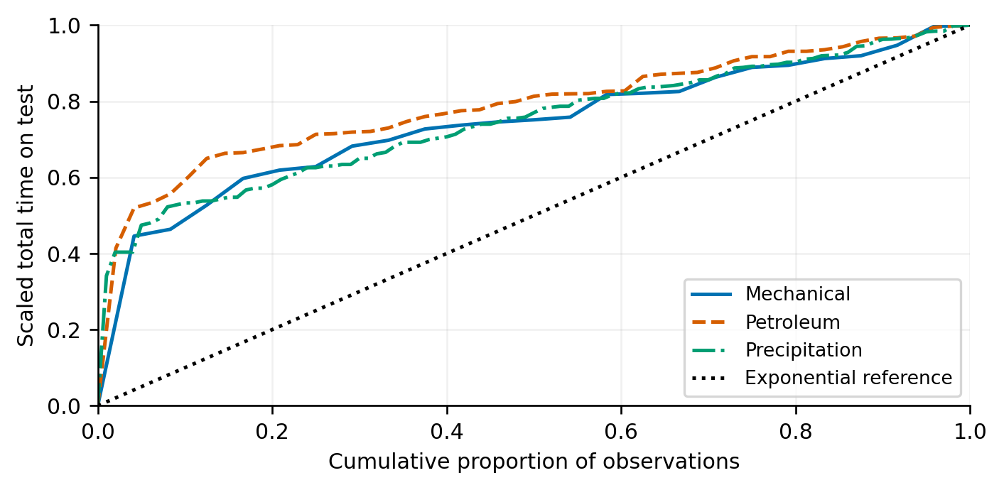
The empirical total-time-on-test coordinates are $u_i=i/n$ and $T_i=[\sum _{j=1}^i{x}_{\left(j\right)}+(n-i\left)x_{\left(i\right)}\right]/\sum _j{x}_j$. These coordinates are unchanged by a common positive multiplier. Figure 1 shows systematic departures from the diagonal for all three samples. This supports examining models with nonconstant hazards, although a small empirical curve cannot identify a complete hazard function.

3.2Mechanical observations

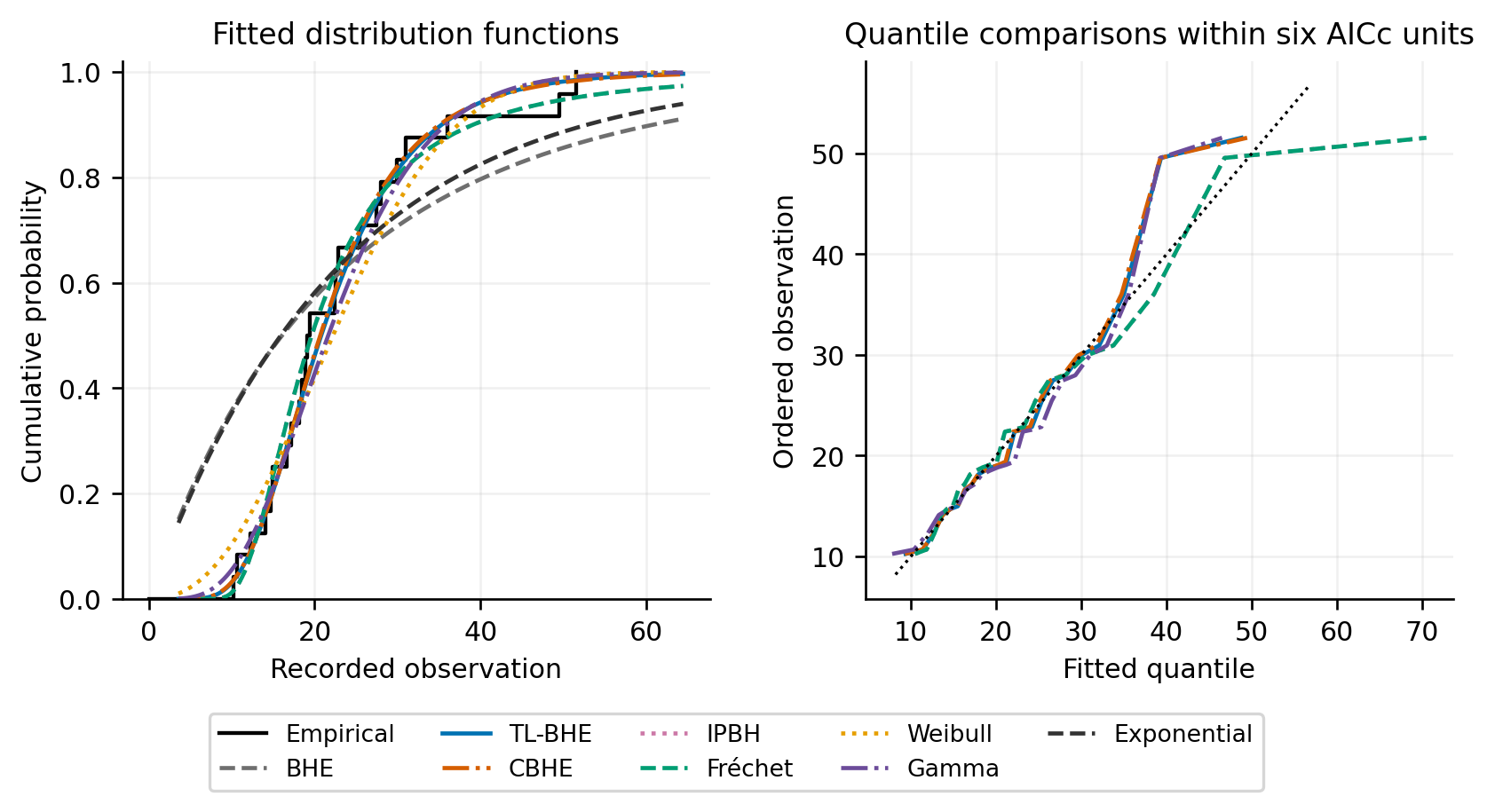
The mechanical sample gives the closest competition among the leading candidates. TL-BHE has the lowest AICc, with IPBH and Fréchet only about 0.31 units higher. Their fitted shapes and upper quantiles are almost identical, as the limiting argument in Section II.B5 suggests. Gamma and CBHE are within four AICc units of the leading fit. Both one-parameter candidates perform poorly under likelihood and held-out scoring. Tables 3–5 report the parameter estimates and comparison measures.

Model	Parameter 1	Parameter 2	Parameter 3
BHE	0.023322	—	—
TL-BHE	15.748103	0.044257	—
CBHE	1.041859	14.554617	0.087466
IPBH	2383.878861	2.734744	—
Fréchet	2.734744	17.179910	—
Weibull	2.308891	26.023002	—
Gamma	5.689749	4.037524	—
Exponential	0.043530	—	—

Parameter order follows Table 1: $\gamma$ for BHE; $\alpha ,\gamma$ for TL-BHE; $\nu ,\xi ,\gamma$ for CBHE; $\alpha ,\beta$ for IPBH; $\kappa ,\sigma$ for Fréchet, Weibull and gamma; and $\lambda$ for exponential. All estimates are interior.

Model	$\widehat{\mathrm{l}}$	AICc	$\Delta$ AICc	Weight	BIC
BHE	-100.8729	203.9277	27.5836	0.0000	204.9239
TL-BHE	-85.8863	176.3440	0.0000	0.2959	178.1287
CBHE	-85.8767	178.9534	2.6093	0.0803	181.2875
IPBH	-86.0418	176.6551	0.3110	0.2533	178.4397
Fréchet	-86.0418	176.6551	0.3110	0.2533	178.4397
Weibull	-88.8910	182.3534	6.0093	0.0147	184.1381
Gamma	-86.9446	178.4607	2.1166	0.1027	180.2454
Exponential	-99.2231	200.6281	24.2841	0.0000	201.6244

Model	ELPD	ELPD deficit	KS	$W^2$	$A^2$
BHE	-101.0451	12.9931	0.3643	0.8167	4.1485
TL-BHE	-88.0521	0.0000	0.1103	0.0256	0.2052
CBHE	-88.0793	0.0272	0.1066	0.0238	0.1914
IPBH	-88.2460	0.1939	0.0891	0.0299	0.2213
Fréchet	-88.2460	0.1939	0.0891	0.0299	0.2213
Weibull	-91.8756	3.8235	0.1436	0.1082	0.7467
Gamma	-89.5372	1.4851	0.1404	0.0568	0.4029
Exponential	-99.4536	11.4015	0.3597	0.7933	3.9769

The ELPD deficit is the best leave-one-out score minus the candidate score. Smaller deficits and fitted discrepancies indicate better performance for their respective targets. We report them separately rather than combining them into a single rank.

TL-BHE has the highest leave-one-out score, but CBHE is only 0.0272 summed log-score units behind and Fréchet is 0.1939 behind. These are small differences for 24 observations. Fréchet and IPBH give the lowest KS statistic, whereas CBHE gives the lowest Anderson–Darling discrepancy. The fitted CDF and quantile plots in Figure 2 show why a distribution preferred by a fitted distance need not lead the predictive-density comparison.

3.3Petroleum observations

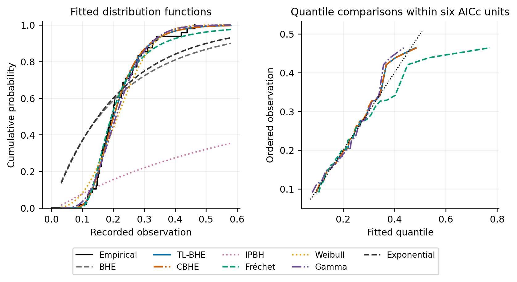
For the petroleum sample, TL-BHE again has the lowest AICc and highest leave-one-out score. CBHE is its closest predictive competitor; its extra parameter increases the information-criterion penalty. Gamma and Fréchet remain within four AICc units. Weibull, exponential and BHE have much lower held-out scores. Tables 6–8 give the numerical results, and Figure 3 shows the fitted CDFs and quantile comparisons.

Model	Parameter 1	Parameter 2	Parameter 3
BHE	2.437068	—	—
TL-BHE	28.057450	5.501949	—
CBHE	0.862349	26.307714	11.470265
IPBH	0.036239	0.932581	—
Fréchet	3.038247	0.172124	—
Weibull	2.747565	0.245226	—
Gamma	7.915268	0.027556	—
Exponential	4.584833	—	—

Parameter order follows Table 1: $\gamma$ for BHE; $\alpha ,\gamma$ for TL-BHE; $\nu ,\xi ,\gamma$ for CBHE; $\alpha ,\beta$ for IPBH; $\kappa ,\sigma$ for Fréchet, Weibull and gamma; and $\lambda$ for exponential. All estimates are interior.

Model	$\widehat{\mathrm{l}}$	AICc	$\Delta$ AICc	Weight	BIC
BHE	21.5294	-40.9718	71.3490	0.0000	-39.1876
TL-BHE	58.2938	-112.3208	0.0000	0.5979	-108.8451
CBHE	58.2628	-109.9802	2.3407	0.1855	-104.9120
IPBH	-17.8944	40.0554	152.3763	0.0000	43.5312
Fréchet	56.4035	-108.5403	3.7805	0.0903	-105.0646
Weibull	52.7422	-101.2177	11.1031	0.0023	-97.7420
Gamma	56.7204	-109.1741	3.1467	0.1240	-105.6984
Exponential	25.0922	-48.0974	64.2234	0.0000	-46.3132

Model	ELPD	ELPD deficit	KS	$W^2$	$A^2$
BHE	21.4148	34.5906	0.3860	1.9628	9.7634
TL-BHE	56.0054	0.0000	0.0896	0.0339	0.2144
CBHE	55.8761	0.1293	0.0871	0.0340	0.2160
IPBH	-17.9781	73.9835	0.6952	8.1717	39.7159
Fréchet	52.4822	3.5232	0.0815	0.0453	0.3731
Weibull	50.0728	5.9326	0.1499	0.1945	1.2295
Gamma	54.4536	1.5518	0.1290	0.0941	0.5559
Exponential	24.9426	31.0628	0.3858	1.9535	9.5709

The ELPD deficit and fitted discrepancies have the same definitions as in Table 5. They assess different features of the fitted models and should be read separately.

The unscaled IPBH fit is constrained by its definition. Every petroleum observation is below one, whereas Proposition 1 requires the model median to exceed one for all positive parameter choices. Its fitted KS statistic is 0.6952 and its leave-one-out deficit is 73.9835. The fitted 0.99 quantile is 143.4314, compared with an observed maximum of 0.4641. These results concern the fixed-reference specification used here; they do not establish that an inverse-power model with a declared physical scale would perform equally poorly.

3.4Precipitation observations

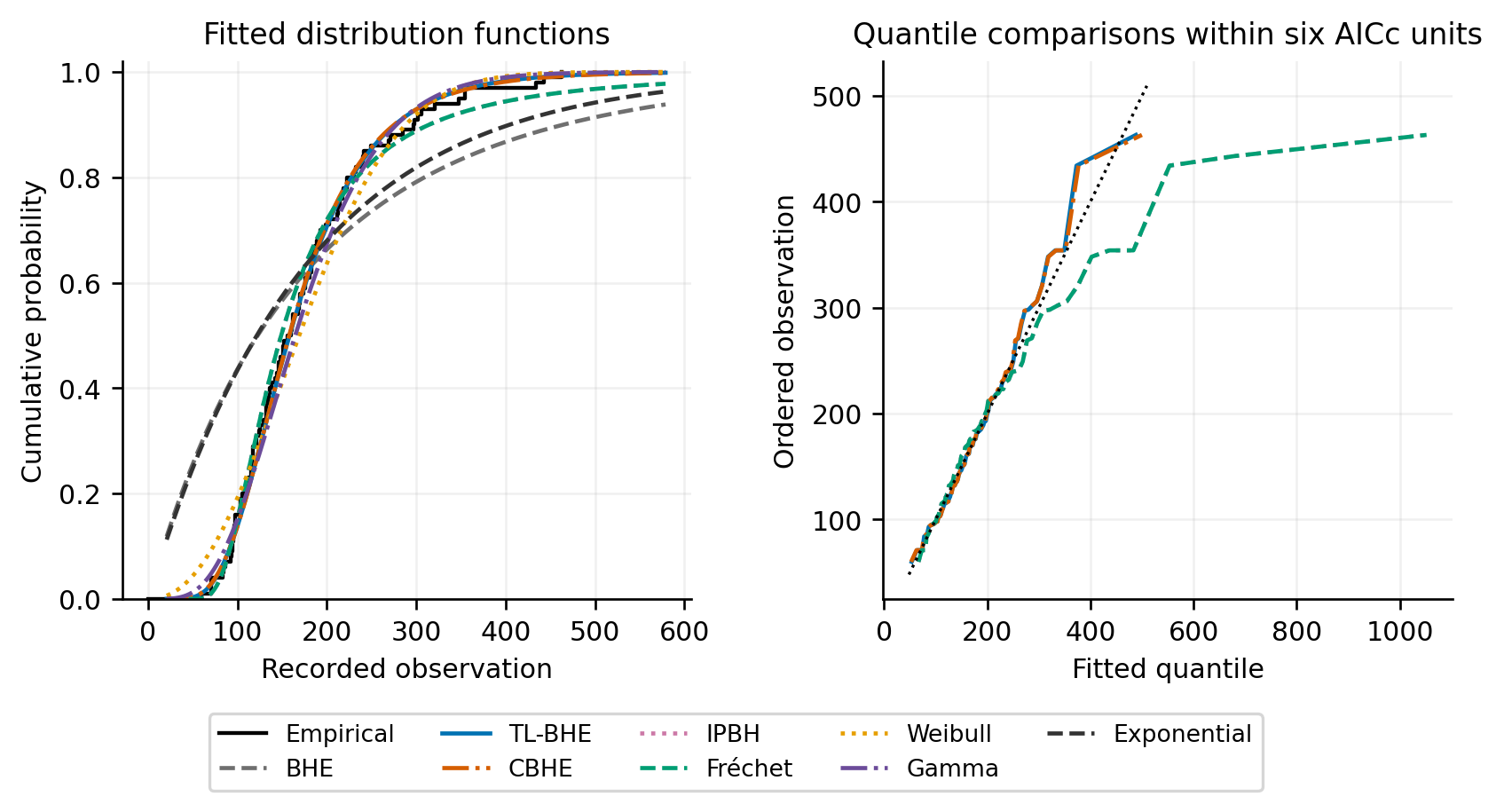
For precipitation, TL-BHE leads the AICc comparison, followed by CBHE. Its leave-one-out score exceeds CBHE by 0.3139 and Fréchet by 2.9078. It also has the lowest KS and Anderson–Darling statistics among these candidates. Tables 9–11 and Figure 4 show greater agreement among the assessment measures than for the mechanical sample. The earlier selection of the examples and the marginal treatment of annual maxima still limit the interpretation.

Model	Parameter 1	Parameter 2	Parameter 3
BHE	0.003055	—	—
TL-BHE	12.786583	0.005392	—
CBHE	0.859905	12.431534	0.011141
IPBH	2.0995e+05	2.522293	—
Fréchet	2.522293	128.833688	—
Weibull	2.250965	199.067375	—
Gamma	5.276326	33.294002	—
Exponential	0.005692	—	—

Parameter order follows Table 1: $\gamma$ for BHE; $\alpha ,\gamma$ for TL-BHE; $\nu ,\xi ,\gamma$ for CBHE; $\alpha ,\beta$ for IPBH; $\kappa ,\sigma$ for Fréchet, Weibull and gamma; and $\lambda$ for exponential. All estimates are interior.

Model	$\widehat{\mathrm{l}}$	AICc	$\Delta$ AICc	Weight	BIC
BHE	-623.6236	1249.2880	113.8294	0.0000	1251.8524
TL-BHE	-565.6674	1135.4586	0.0000	0.6640	1140.5452
CBHE	-565.8140	1137.8780	2.4194	0.1981	1145.4435
IPBH	-568.1275	1140.3787	4.9201	0.0567	1145.4653
Fréchet	-568.1275	1140.3787	4.9201	0.0567	1145.4653
Weibull	-576.0977	1156.3190	20.8605	0.0000	1161.4057
Gamma	-568.9698	1142.0634	6.6048	0.0244	1147.1500
Exponential	-616.8607	1235.7623	100.3037	0.0000	1238.3266

Model	ELPD	ELPD deficit	KS	$W^2$	$A^2$
BHE	-623.7963	56.2176	0.3443	3.1208	16.0839
TL-BHE	-567.5787	0.0000	0.0529	0.0361	0.2821
CBHE	-567.8926	0.3139	0.0539	0.0374	0.2886
IPBH	-570.4865	2.9078	0.0605	0.0704	0.5212
Fréchet	-570.4865	2.9078	0.0605	0.0704	0.5212
Weibull	-578.6873	11.1087	0.0950	0.2692	1.8650
Gamma	-571.1054	3.5268	0.0610	0.1134	0.7868
Exponential	-617.0874	49.5088	0.3410	3.0042	15.2845

ELPD deficits and fitted discrepancies are defined as in Table 5. Each measures a different feature of performance.

The profiled IPBH fit is close to Fréchet, with shape 2.5223 and a large first parameter. Its parameter pair differs substantially from the retained source pair. Profiling improves the likelihood under the same IPBH density; Section III.E examines the difference explicitly.

3.5Audit of the source inverse power solution

Table 12 compares the retained source log likelihoods with the new profile solutions. The mechanical and petroleum calculations agree with the source values to their reported precision. For precipitation, the profile gives a higher likelihood. Both parameter pairs are evaluated with the same unscaled IPBH formula and the same 100 observations.

Sample	Reported log likelihood	Profile log likelihood	Improvement
Mechanical	-86.0418	-86.0418	0.0000
Petroleum	-17.8944	-17.8944	0.0000
Precipitation	-581.6162	-568.1275	13.4887

The precipitation source pair is $(\alpha ,\beta )=(2980.96,1.63858)$, while the profile estimate is approximately $(209946.96,2.52229)$. Direct evaluation at the printed source parameters gives log likelihood −581.6162, whereas the profile pair gives −568.1275. The improvement is 13.4887. Since the parameter count is unchanged, the corresponding AICc improvement is 26.9774. The earlier pair is therefore not the maximizer found for the specified density under the present profile search. We do not infer which stopping rule or starting point produced it.

The difference changes how competitive IPBH appears in the precipitation comparison. We use the profiled solution in the model-comparison tables and retain the earlier values in Table 12 as an explicit numerical benchmark. A correctly evaluated likelihood at a reported parameter pair is not, by itself, evidence that the pair maximizes that likelihood.

3.6Candidate duplication and relative support

In the mechanical sample, the separate IPBH and Fréchet weights are each approximately 0.2533, while the TL-BHE weight is 0.2959. Removing the nearly duplicate IPBH entry and renormalizing the same remaining likelihood weights would raise the TL-BHE weight to 0.3962. In precipitation the corresponding change is from 0.6640 to 0.7040. These changes require no refitting and no improvement in any model. They arise because the denominator in the weight expression changes.

Akaike weights must therefore be interpreted with the candidate list in view. Two nearly identical fitted curves can divide the support associated with similar predictions. We retain IPBH and Fréchet because they have distinct definitions and behave very differently for the petroleum observations, while making their near duplication in the other examples explicit.

3.7Upper-tail and measurement-scale sensitivity

3.7.1Fitted upper quantiles

Model	Mech Q95	Mech Q99	Petro Q95	Petro Q99	Precip Q95	Precip Q99
BHE	82.4587	136.1748	0.7891	1.3031	629.4509	1039.4948
TL-BHE	41.2489	55.1868	0.3709	0.4849	324.3808	438.0510
CBHE	41.2933	56.5034	0.3702	0.4896	325.5160	446.2492
IPBH	50.8987	92.3748	24.4690	143.4314	418.2586	798.1680
Fréchet	50.8987	92.3748	0.4575	0.7823	418.2586	798.1680
Weibull	41.8538	50.4214	0.3656	0.4275	324.1070	392.3283
Gamma	40.7582	51.0622	0.3593	0.4376	317.3816	400.3613
Exponential	68.8195	105.7923	0.6534	1.0044	526.2603	808.9902

Table 13 shows that the mechanical TL-BHE 0.99 quantile is 55.1868, whereas Fréchet and IPBH give 92.3748. Both heavier-tailed alternatives are only about 0.31 AICc units from the leading fit. Their quantile exceeds the TL-BHE value by about 67.4%. The observed maximum, 51.56, is close to the TL-BHE quantile and well below the two heavier-tailed estimates. A close likelihood comparison consequently leaves a substantial choice of extrapolated tail values.

For petroleum, TL-BHE gives a 0.99 quantile of 0.4849, gamma gives 0.4376 and Fréchet gives 0.7823. These values are much closer to the observed scale than the unscaled IPBH prediction. For precipitation, TL-BHE and CBHE give 438.0510 and 446.2492, whereas the newly optimized IPBH and Fréchet fits give approximately 798.1680. The likelihood penalty for the heavier-tailed alternatives is larger here than in the mechanical sample, but their extrapolation still illustrates the role of tail assumptions.

These are fitted marginal quantiles. Their uncertainty includes parameter estimation, choice of candidate and adequacy of the assumed tail form. Table 13 does not give confidence limits. For precipitation, interpreting a fitted quantile as a calibrated engineering return level would also require evidence about stationarity and serial independence.

3.7.2Sensitivity to the candidate support threshold

Sample	Threshold c	Models	Minimum Q99	Maximum Q99	Ratio
Mechanical	2	3	55.1868	92.3748	1.674
Mechanical	4	5	51.0622	92.3748	1.809
Mechanical	6	5	51.0622	92.3748	1.809
Petroleum	2	1	0.4849	0.4849	1.000
Petroleum	4	4	0.4376	0.7823	1.788
Petroleum	6	4	0.4376	0.7823	1.788
Precipitation	2	1	438.0510	438.0510	1.000
Precipitation	4	2	438.0510	446.2492	1.019
Precipitation	6	4	438.0510	798.1680	1.822

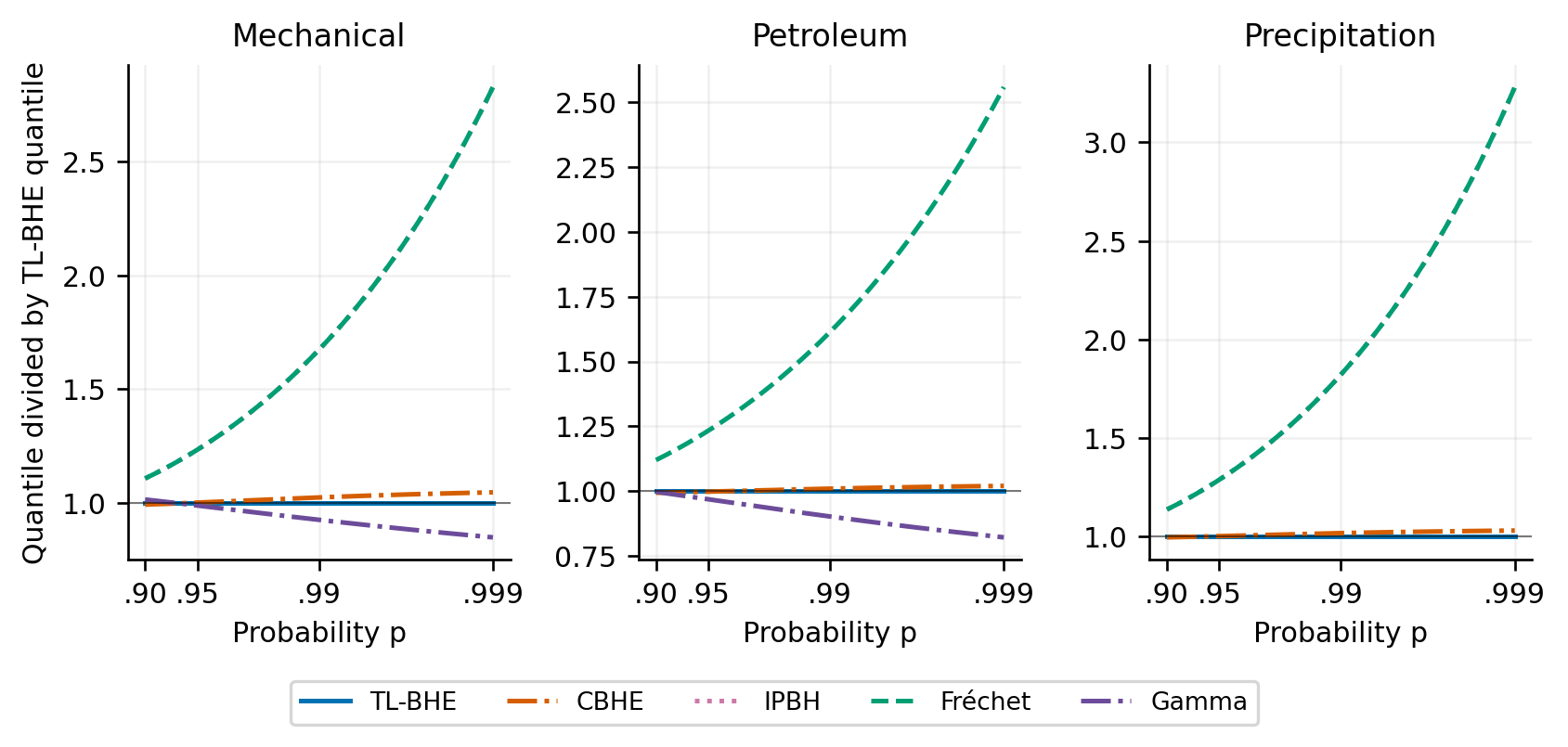
Table 14 shows how the range changes with the AICc threshold. For mechanical data, substantially different upper quantiles already occur at a threshold of two. The petroleum range widens between thresholds two and four. The precipitation range is narrow at four and widens markedly at six, when Fréchet and IPBH enter the set. Figure 5 traces the corresponding quantile ratios across upper probabilities. Reporting both the threshold and the individual quantiles makes this dependence visible.

3.7.3Controlled changes of the numerical scale

Sample	Multiplier a	Common AICc	IPBH rank	KS	Common Q99
Mechanical	0.01	244.3686	8	0.6732	13564.6320
Mechanical	0.10	176.5631	2	0.0870	90.4163
Mechanical	1.00	176.6551	2	0.0891	92.3748
Mechanical	10.00	176.6551	2	0.0891	92.3748
Mechanical	100.00	176.6551	2	0.0891	92.3748
Petroleum	0.01	168.9783	8	0.8151	2.1413e+10
Petroleum	0.10	124.5337	8	0.7936	1.7311e+06
Petroleum	1.00	40.0554	8	0.6952	143.4314
Petroleum	10.00	-108.8573	4	0.0807	0.7685
Petroleum	100.00	-108.5403	4	0.0815	0.7823
Precipitation	0.01	1138.6398	3	0.0586	726.2955
Precipitation	0.10	1140.3786	3	0.0605	798.1687
Precipitation	1.00	1140.3787	3	0.0605	798.1680
Precipitation	10.00	1140.3787	3	0.0605	798.1680
Precipitation	100.00	1140.3787	3	0.0605	798.1680

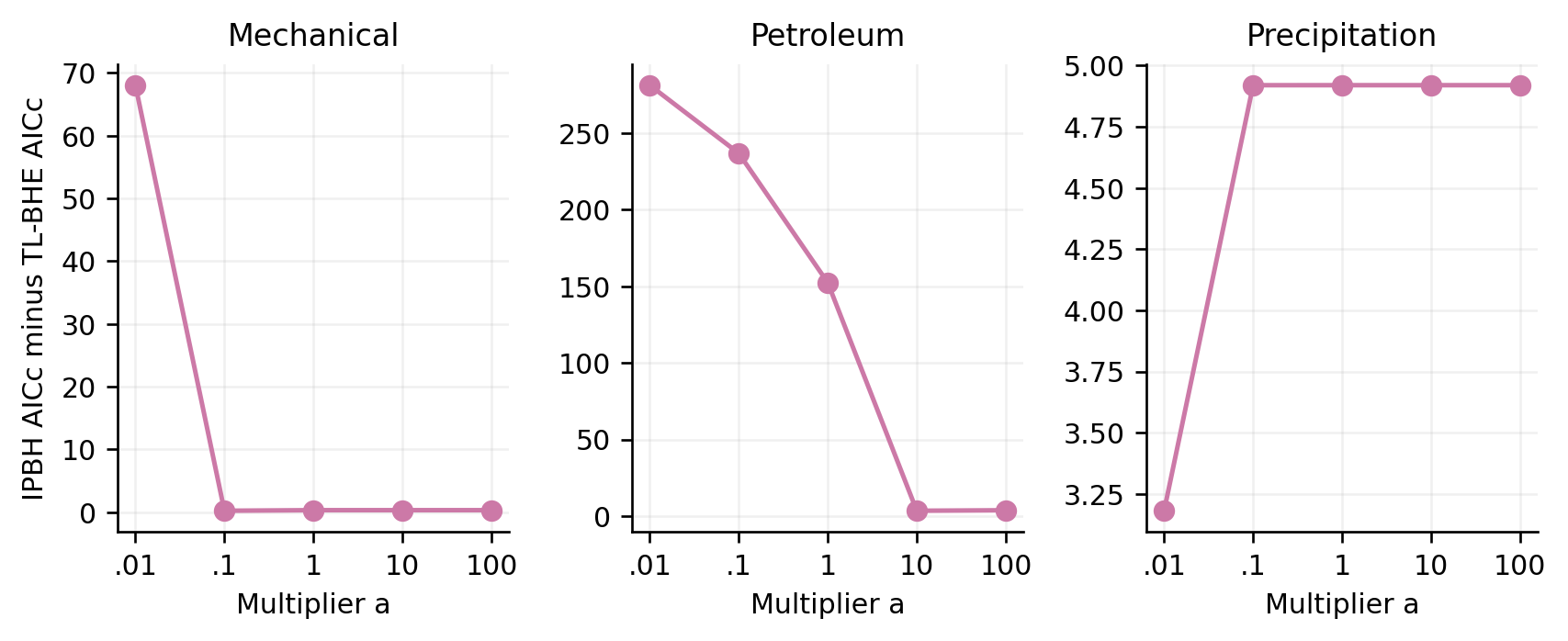
The numerical-scale experiment in Table 15 exposes the fixed reference in the IPBH formula. Multiplying the mechanical observations by 0.01 puts every value below one and moves IPBH to rank eight. At multipliers of 0.1 and above, it fits much more like Fréchet. For petroleum, its rank is eight at multipliers 0.01, 0.1 and 1, and improves to four at 10 and 100. Even after converting the quantiles back, their values vary by orders of magnitude. The seven scale families preserve their corrected likelihoods and fitted CDFs under the same conversions.

The precipitation example shows a smaller effect because most original values are far above the implicit reference. At a multiplier of 0.01, the corrected IPBH AICc is 1138.6398, compared with approximately 1140.3787 on the original scale. At larger multipliers, the fit approaches the Fréchet result. Figure 6 shows these changes relative to the invariant TL-BHE comparison. The experiment changes the physical reference represented by the unscaled formula; it does not change the physical observations.

Independent refits of the seven scale families at $a=0.01$ and $a=100$ agree with their transformed full-sample likelihoods within ${10}^{-6}$. Their fitted CDF differences are below ${10}^{-10}$. These checks distinguish an optimizer or Jacobian error from the structural lack of closure proved for unscaled IPBH. Declaring and converting a physical reference $c$ as in Section II.B4 restores the appropriate unit relation.

3.7.4Which observations favour a heavier tail

For each observation, let $d_i$ be its TL-BHE held-out log density minus its Fréchet held-out log density. The sum of these contributions equals the difference in the two ELPD scores. A positive contribution favours TL-BHE for that value; a negative contribution favours Fréchet.

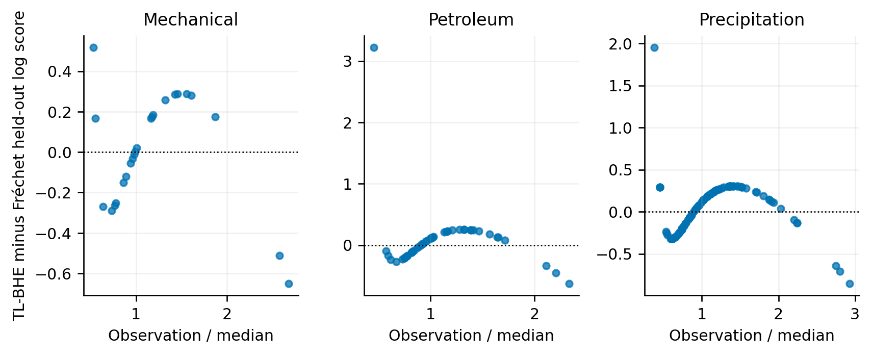
Figure 7 separates the aggregate score into observation-level contributions. Some large observations favour Fréchet even when the summed score favours TL-BHE. The log score evaluates the whole fitted density, whereas a high quantile concerns a specific tail region. This distinction matters most in the mechanical sample, where the two aggregate scores are close.

4Discussion

The results identify three issues that can be missed in a conventional model-ranking table. The most direct is the fixed reference in the IPBH specification. Its median constraint explains the petroleum result before any fitting is attempted. The lack of scale closure then explains why applying the raw formula in different numerical units changes its apparent performance. These conclusions follow from the CDF and are supported by the controlled refits.

For physical measurements, the IPBH argument should be made dimensionless through a declared reference value. Converting that reference together with the observations preserves the physical model. Estimating the reference instead changes the model and adds a fitted parameter. The distinction should be stated when comparing information criteria or upper quantiles.

Choosing a unit conversion because it improves the raw IPBH fit would adapt the reference to the sample. Its effect would have to be accounted for in model assessment. Our experiment holds the numerical reference at one to expose the consequence of an undeclared convention. It provides an audit of the specification, rather than a procedure for choosing favourable units.

The precipitation calculation raises a separate numerical concern. Conditional maximization in the first IPBH parameter and profiling over the second produce a substantially better likelihood than the retained source pair. Checking scores, using exact conditional reductions and comparing alternative starts can reveal an inferior fit that an optimizer success message alone would miss.

The tail comparison has a direct practical consequence. The near-leading mechanical Fréchet and IPBH fits predict a much larger 0.99 quantile than TL-BHE. For precipitation, changing the AICc threshold from four to six brings similarly large upper quantiles into the sensitivity range. A model selected for its overall fit should therefore be accompanied by the tail quantities relevant to its intended use.

The empirical evidence remains limited to three previously screened datasets and the stated candidate families. Recorded ties are treated using continuous densities because the recording intervals have not been verified. Leave-one-out refitting assesses marginal density prediction under an exchangeable working sample. It does not establish stationarity or temporal independence of the precipitation series. The study also does not estimate confidence-interval coverage or formal goodness-of-fit rejection rates.

Further work could examine independently selected samples and prespecified physical reference scales. Simulation would help assess selection of lighter and heavier tails, bias and interval coverage of upper quantiles, and the effect of recording intervals. Environmental prediction would additionally require verified units, dependence assessment and evaluation in time order. These steps would test questions that the present case studies leave open.

5Conclusion

For these three samples, TL-BHE has the lowest AICc and highest leave-one-out score among the eight candidates. The differences from several alternatives are small, especially for the mechanical data. Near-leading models there give 0.99 quantiles of approximately 55.19 and 92.37, so agreement in overall fit does not imply agreement about the upper tail.

The unscaled IPBH median exceeds one, and its two shape parameters cannot absorb a nontrivial change of numerical units. The refitting experiment demonstrates the resulting sensitivity, while properly transformed scale families preserve their fitted probabilities and corrected likelihoods. The precipitation audit also shows the value of checking likelihood maximization. In applied comparisons, a declared reference scale, a checked fitting procedure and explicit upper-tail sensitivity are needed to interpret what the preferred model can support.

Funding

The publication costs are self-funded. The submitting author will personally pay the journal’s article processing charge.

Conflict of Interest

The author declares no competing interests.

Data Availability

The observation vectors are reproduced in Appendix B. Appendix C specifies the numerical fitting and validation procedures. All model-comparison, leave-one-out and unit-sensitivity results were calculated from these vectors for the present analysis. The retained source parameter pairs and log likelihoods used as benchmarks are reported separately in Section III.E.

References

1. [1]Yadav AS, Altun E, Yousof HM. Burr–Hatke exponential distribution: A decreasing failure rate model, statistical inference and applications. Annals of Data Science. 2021;8:241–260. https://doi.org/10.1007/s40745-019-00213-8
2. [2]Afify AZ, Aljohani HM, Alghamdi AS, Gemeay AM, Sarg AM. A new two-parameter Burr–Hatke distribution: Properties and Bayesian and non-Bayesian inference with applications. Journal of Mathematics. 2021;2021:1061083. https://doi.org/10.1155/2021/1061083
3. [3]Abubakari AG, Anzagra L, Nasiru S. Chen Burr-Hatke exponential distribution: Properties, regressions and biomedical applications. Computational Journal of Mathematical and Statistical Sciences. 2023;2(1):80–105. https://doi.org/10.21608/cjmss.2023.190993.1003
4. [4]Anyiam KE, Alghamdi FM, Nwaigwe CC, Aljohani HM, Obulezi OJ. A new extension of Burr-Hatke exponential distribution with engineering and biomedical applications. Heliyon. 2024;10(19):e38293. https://doi.org/10.1016/j.heliyon.2024.e38293
5. [5]Akaike H. A new look at the statistical model identification. IEEE Transactions on Automatic Control. 1974;19(6):716–723. https://doi.org/10.1109/TAC.1974.1100705
6. [6]Schwarz G. Estimating the dimension of a model. The Annals of Statistics. 1978;6(2):461–464. https://doi.org/10.1214/aos/1176344136
7. [7]Hurvich CM, Tsai CL. Regression and time series model selection in small samples. Biometrika. 1989;76(2):297–307. https://doi.org/10.1093/biomet/76.2.297
8. [8]Burnham KP, Anderson DR. Model selection and multimodel inference: A practical information-theoretic approach. 2nd ed. New York: Springer; 2002. https://doi.org/10.1007/b97636
9. [9]Stone M. An asymptotic equivalence of choice of model by cross-validation and Akaike’s criterion. Journal of the Royal Statistical Society Series B. 1977;39(1):44–47. https://doi.org/10.1111/j.2517-6161.1977.tb01603.x
10. [10]NIST/SEMATECH. e-Handbook of statistical methods [Internet]. Gaithersburg: National Institute of Standards and Technology [cited 2026 Oct 1]. Available from: https://www.itl.nist.gov/div898/handbook/
11. [11]Corless RM, Gonnet GH, Hare DEG, Jeffrey DJ, Knuth DE. On the Lambert W function. Advances in Computational Mathematics. 1996;5:329–359. https://doi.org/10.1007/BF02124750
12. [12]Mandouh RM, Mohamed MA. Log-weighted Pareto distribution and its statistical properties. Journal of Data Science. 2020;18(1):161–189. https://doi.org/10.6339/JDS.202001_18(1).0009
13. [13]Murthy DNP, Xie M, Jiang R. Weibull models. Hoboken: Wiley; 2004.
14. [14]ZeinEldin RA, Haq MAU, Hashmi S, Elsehety M, Elgarhy M. Type II half logistic Kumaraswamy distribution with applications. Journal of Function Spaces. 2020;2020:1343596. https://doi.org/10.1155/2020/1343596
15. [15]Imran M, Tahir MH, Jamal F. DataSetsUni: A collection of univariate data sets [software]. Version 0.1. CRAN; 2023. Available from: https://cran.r-project.org/package=DataSetsUni
16. [16]Anderson TW, Darling DA. Asymptotic theory of certain goodness-of-fit criteria based on stochastic processes. The Annals of Mathematical Statistics. 1952;23(2):193–212. https://doi.org/10.1214/aoms/1177729437

Appendix A. Additional derivative details

Chain rule derivatives for CBHE

Write $A_i=\partial \log g_i/\partial \gamma$ and $D_i=\partial \log G_i/\partial \gamma$. From the baseline,

The three CBHE scores follow by differentiating its compact log likelihood:

The derivative of the log normalizer contributes the final term of $U_{\nu }$. Omitting it changes the likelihood equations. On logarithmic parameters, the corresponding score components are $\nu U_{\nu }$, $\xi U_{\xi }$ and $\gamma U_{\gamma }$. The minimizing code uses their negatives and divides the objective and gradient by $n$. This positive scaling leaves its maximizer unchanged.

Profile and quantile identities

The IPBH second-shape score, useful for checking a profile solution, is

When the conditional first-shape score is zero, differentiating the profile likelihood in $\beta$ gives this same score. The derivative through $\widehat{\alpha }\left(\beta \right)$ vanishes because it is multiplied by $U_{\alpha }$. This explains why the scalar profile retains the joint likelihood stationary equations.

For completeness, an algebraic IPBH quantile can be derived from $p=e^{-\alpha u}/(1+u)$. Put $t=\alpha (1+u)$; then $t{e}^t=\alpha e^{\alpha }/p$, so

The root form used computationally is equivalent and is more stable for large $\alpha$. For reference-scale notation, a fixed $c$ multiplies this dimensionless quantile. This also verifies that converting $c$ together with the data preserves the resulting physical quantile.

Appendix B. Observation vectors

Tables 16–18 list the mechanical, petroleum and precipitation observations, respectively, in their source order. They retain the original numerical scales and all repeated entries.

1	2	3	4	5	6
30.94	18.51	16.62	51.56	22.85	22.38
19.08	49.56	17.12	10.67	25.43	10.24
27.47	14.70	14.10	29.93	27.98	36.02
19.40	14.97	22.57	12.26	18.14	18.84

1	2	3	4	5	6
0.0903296	0.203654	0.204314	0.280887	0.197653	0.328641
0.148622	0.162394	0.262727	0.179455	0.326635	0.230081
0.183312	0.150944	0.200071	0.191802	0.154192	0.464125
0.117063	0.148141	0.14481	0.133083	0.276016	0.420477
0.122417	0.228595	0.113852	0.225214	0.176969	0.200744
0.167045	0.231623	0.291029	0.341273	0.438712	0.262651
0.189651	0.172567	0.240077	0.311646	0.163586	0.182453
0.164127	0.153481	0.161865	0.276016	0.253832	0.200447

1	2	3	4	5	6	7	8	9	10
239	232	434	85	302	174	170	121	193	168
148	116	132	132	144	183	223	96	298	97
116	146	84	230	138	170	117	115	132	125
156	124	189	193	71	176	105	93	354	60
151	160	219	142	117	87	223	215	108	354
213	306	169	184	71	98	96	218	176	121
161	321	102	269	98	271	95	212	151	136
240	162	71	110	285	215	103	443	185	199
115	134	297	187	203	146	94	129	162	112
348	95	249	103	181	152	135	463	183	241

Appendix C. Computational specification

The calculations use Python, NumPy 2.3.5 and SciPy 1.17.0. All numerical fits, profile grids and held-out comparisons are deterministic. No random simulation or random seed is required for the reported analysis.

The BHE rate and classical shape equations use bracketed roots with a coordinate tolerance of ${10}^{-12}$. The TL-BHE log-rate profile is bracketed using 40 points between −10 and 4 on the median-standardized scale and refined to a coordinate tolerance of ${10}^{-11}$. The IPBH log-shape profile uses 45 points from −7 to 3.5; its conditional first-shape root is solved inside the explicit bracket in Section II.C4. IPBH uses the raw observation values, so median standardization is not substituted into its formula.

For full-sample CBHE fits, $\nu$ starts at 0.001, 0.03, 0.3, 1, 3, 10 and 60. The $\xi$ starts are 0.5, 1 and 2 times the TL-BHE shape, and the standardized rate starts at twice its fitted rate. The computational safeguards are approximately ${10}^{-6}\le \nu \le {10}^3$, ${10}^{-3}\le \xi \le {10}^4$ and ${10}^{-6}\le \gamma \le {10}^3$ on the standardized scale. They are numerical search limits, not boundaries of the probability model.

Quasi-Newton optimization allows 1,200 iterations with function tolerance ${10}^{-14}$ and gradient tolerance ${10}^{-9}$. Simplex refinement allows 1,500 iterations with coordinate tolerance ${10}^{-9}$ and function tolerance ${10}^{-13}$. Final scaled gradient checks use ${10}^{-5}$ as the acceptance threshold. The best admissible objective value is retained across the searches. Full-sample and leave-one-out solutions are interior under these safeguards.

Leave-one-out CBHE fitting begins at the full-sample estimate and uses three additional first-shape starts, 0.03, 1 and 10, with the conditional TL-BHE shape and rate from the training sample. Identical held-out entries reuse the same training fit but retain their separate score contributions. Every training sample contains exactly one fewer observation. Unit checks use fixed multipliers 0.01, 0.1, 1, 10 and 100. Quantiles are inverted at full numerical precision before table rounding.

Independent checks integrate each density to one, compare it with a numerical CDF derivative and verify $F\left(Q\right(p\left)\right)=p$ at seven probabilities from 0.00001 to 0.99999. The largest absolute density-derivative discrepancy is below ${10}^{-7}$, the inversion discrepancy below ${10}^{-8}$, and the CBHE analytical-gradient discrepancy below ${10}^{-5}$. Transformed and independently refitted scale-family likelihoods agree within ${10}^{-6}$. All tables round final values after calculation; scientific notation is used when ordinary decimals would obscure very large or very small values.