Patient-Level Deep Fusion, Radiomics, and Ensemble Learning for CT-Based Differentiation of Multiple Primary Lung Cancers

1Introduction

Lung cancer remains a leading cause of cancer-related mortality worldwide, with adenocarcinoma and squamous cell carcinoma accounting for the majority of cases [1]. With improved chest CT technology and health surveillance, patients presenting with more than one pulmonary lesion are encountered more frequently, and multiple primary lung cancers (MPLCs) are estimated to represent roughly 0.8%–16% of confirmed lung cancer cases [2], [3].

In clinical practice, patients with multiple pulmonary nodules fall into three broad groups: MPLCs, intrapulmonary metastases (IPMs), and multiple benign pulmonary lesions (MBPLs). The distinction matters because the management differs: benign lesions are generally monitored or treated symptomatically, certain MPLCs respond well to surgical resection, whereas IPMs usually offer limited surgical options and a poorer prognosis [4]–[6]. Current diagnosis relies on the 2013 ACCP criteria [7] and comprehensive histologic assessment [8], which depend on invasive sampling and subjective interpretation.

CT-based radiomics has been used to separate MPLC from IPM, for example with reported AUCs of 0.889 [9] and, in a pairwise lesion-relation model, 0.983 on training data [10]. Hybrid approaches that combine radiomic and deep features have also shown strong performance for nodule malignancy prediction [11]. Deep learning more broadly has shown promise in lung cancer detection, segmentation, and staging [15], [16]. A recent study compared several pretrained 2D architectures for three-class MPLC/IPM/MBPL discrimination using image-level slice classification [14]; however, such slice-level designs can leak information between train and test splits and do not model a patient as a set of lesions.

In this work we address these gaps with a patient-level framework. Our contributions are:

• a deep fusion model combining 2D multiple-instance learning over slices, a 3D volumetric branch, and radiomic features;
• radiomics-based Random Forest and XGBoost classifiers as strong, interpretable baselines;
• a soft-voting ensemble of the above models; and
• a comprehensive evaluation using accuracy, precision, recall, F1-score, specificity, ROC-AUC, and confusion matrices.

2Related work

Radiomics for MPLC and IPM. Radiomic models built on CT features and clinical variables have been used to differentiate MPLC from IPM [9], [10]. Multidisciplinary algorithms that integrate histology, molecular markers such as EGFR and ALK, and imaging have also improved classification and prognostic value [13], and staged algorithms using CT and PET/CT findings have reported an IPM diagnostic accuracy of 88.9% [12].

Deep learning on CT. Convolutional networks such as ResNet [17], DenseNet [18], and EfficientNet [19], as well as transformer and state-space architectures [20]–[22], have been widely applied to medical imaging. Liufu et al. [14] compared six pretrained backbones for MPLC/IPM/MBPL classification and reported a five-fold cross-validated macro-AUC of 0.946, while noting that image-level splitting and a modest dataset were limitations.

Multiple-instance learning and ensembles. Attention-based multiple-instance learning treats a patient as a bag of slices or lesions and learns which instances are informative [23]. Tree ensembles such as Random Forest [24] and gradient boosting [25] are well suited to tabular radiomic features, which are typically high-dimensional relative to sample size.

3Proposed methodology

3.1Dataset

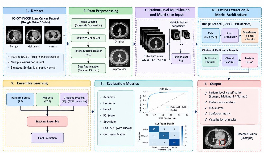
The IQ-OTHNCCD lung cancer dataset was used for the experimental evaluation of the proposed lung cancer classification model. The dataset contains 1,097 CT images distributed among three classes: Normal (416 images), Benign (120 images), and Malignant (561 images). All images are stored in JPEG format with a resolution of 512 × 512 pixels and RGB color representation. The three-class organization enables the model to distinguish normal lung CT scans from benign and malignant cases (Table 1).

Class	Number of Images
Normal	416
Benign	120
Malignant	561
Total	1097

3.2Data preprocessing

Before model training, the CT images were subjected to a standardized preprocessing pipeline to ensure consistent input characteristics. First, the images were checked for readability and organized according to their corresponding class labels. Each image was resized from 512 × 512 pixels to the input resolution required by the proposed deep-learning model. Pixel values were then normalized to a suitable numerical range to improve training stability. To improve model generalization and reduce overfitting, data augmentation such as horizontal flipping, small rotations, scaling, and translation can be applied to the training images only. Finally, the dataset was divided into training, validation, and testing subsets using a stratified splitting strategy, ensuring that all three classes were represented in each subset. Importantly, augmentation was not applied to the validation or test sets so that the reported performance reflects the model’s performance on unseen images. The overall workflow is shown in Fig. 1.

3.3Patient-level bag construction and radiomic feature extraction

Radiomic features (shape, first-order statistics, and texture families such as GLCM, GLRLM, and GLSZM) were extracted from segmented lesions using the PyRadiomics library [26]. Features were standardized using training-set statistics, and highly correlated or low-variance features were removed prior to modeling. Algorithm 1 summarizes the construction of patient-level bags, radiomic feature aggregation, and the patient-level data split.

Algorithm 1. Patient-level bag construction and radiomics feature extraction

Require: CT image set I with class labels; slices per bag K = 8; image size S = 224; optional patient map M and clinical table C
Ensure: Bags {(Vi, ri, yi)}i=1N; splits Dtr, Dva, Dte; scaled features r̃i
 1: Set the random seed to 42
 2: Collect all images in I; derive each label y from its folder name
 3: if M is available then
 4:     Assign real patient IDs from M
 5: else
 6:     Sort slices of each class in natural filename order
 7:     Group every K consecutive slices into one pseudo-patient
 8: end if
 9: for all patients p with at least 2 slices do
10:     if |p| ≥ K then
11:         Select K slices at evenly spaced indices
12:     else
13:         Pad by repeating the last slice until |p| = K
14:     end if
15:     Load slices as grayscale, resize to S × S, stack into V ∈ RK×S×S
16: end for
17: for all bags V do
18:     for all slices xk ∈ V do
19:         fk ← [first-order statistics, Otsu foreground ratio, GLCM features, LBP histogram]
20:     end for
21:     r ← [μ(f1:K); σ(f1:K); max(f1:K)]
22:     if C is available then
23:         r ← [r; cp]
24:     end if
25: end for
26: Stratified patient-level split: 70% train, 15% validation, 15% test
27: Fit StandardScaler on Dtr only; compute r̃i for all bags
28: return Dtr, Dva, Dte, {r̃i}

3.4Deep fusion model

The deep fusion model has three branches whose outputs are concatenated before classification:

• 2D-MIL branch: each patient is treated as a bag of axial slices. A pretrained 2D CNN encodes each slice, and an attention-based pooling operator [23] aggregates the slice embeddings into a patient-level representation:

where h_k is the embedding of slice k, and w, V are learnable parameters.

• 3D branch: a 3D convolutional encoder processes the volumetric crop and yields z_3D.
• Radiomics branch: a small multilayer perceptron maps the standardized radiomic vector to z_rad.

The fused representation z = [z_2D; z_3D; z_rad] is passed to a fully connected classifier trained with cross-entropy loss, the AdamW optimizer, a learning-rate scheduler, and early stopping on validation performance. The complete training procedure is given in Algorithm 2.

Algorithm 2. Training of the deep fusion network (2D-MIL + 3D CNN + radiomics)

Require: Dtr, Dva; epochs E = 25; learning rate η = 10−4; patience P = 6; batch size 4
Ensure: Best fusion model fθ*
 1: Initialize ImageNet-pretrained ResNet-18 (no classifier) as slice encoder φ2D; initialize attention-MIL, 3D CNN φ3D, radiomics MLP φrad, and fusion head
 2: Class weights wc = Ntr/(C · nc); loss L: weighted cross-entropy with label smoothing 0.05; AdamW (weight decay 10−4) with cosine annealing
 3: F1best ← −1, wait ← 0
 4: for e = 1 to E do
 5:     for all mini-batches (V, r̃, y) ∈ Dtr do
 6:         Augment V (horizontal/vertical flips, random intensity scaling)
 7:         hk ← φ2D(xk) ∈ R512 for k = 1, . . . , K
 8:         z2D ← Σk=1K akhk with ak from Eq. (1)
 9:         z3D ← φ3D(V); zrad ← φrad(r̃)
10:         ŷ ← Head([z2D; z3D; zrad])
11:         Update θ by back-propagating L(ŷ, y)
12:     end for
13:     Step the scheduler; compute macro-F1 F1val on Dva
14:     if F1val > F1best then
15:         F1best ← F1val; θ* ← θ; wait ← 0
16:     else
17:         wait ← wait + 1
18:         if wait ≥ P then
19:             break
20:         end if
21:     end if
22: end for
23: return fθ*

3.5Radiomics-based machine learning models

Random Forest [24] and XGBoost [25] classifiers were trained on the radiomic feature vectors. Hyperparameters (e.g., number of trees, tree depth, learning rate) were tuned using validation performance.

3.6Proposed XGBoost-based radiomics architecture

The proposed XGBoost (Radiomics) architecture is designed to detect and classify Multiple Primary Lung Cancers (MPLC) from chest CT images by converting lesion-level imaging characteristics into a compact, discriminative radiomic representation. After CT image preprocessing, including grayscale conversion, resizing to 224 × 224, intensity normalization to [0, 1], and augmentation, the suspicious lung-lesion regions are considered as regions of interest (ROIs). From each ROI, a radiomic feature vector x_i = [x_i1, x_i2, . . . , x_id] is extracted, incorporating first-order intensity, shape, texture, and higher-order texture descriptors such as GLCM, GLRLM, GLSZM and related statistical features. Since a patient may contain multiple lesions and multiple CT slices, the lesion-level features are aggregated to obtain a patient-level representation, for example,

where L_p denotes the number of lesions associated with patient p, and Agg(·) represents an appropriate aggregation operation such as mean, maximum, or statistical pooling across lesions. The resulting patient-level radiomic vector is supplied to the Extreme Gradient Boosting (XGBoost) classifier. XGBoost constructs an ensemble of T regression trees, where the prediction can be expressed as

with f_t representing the t-th decision tree and yˆ_p denoting the predicted probabilities for the three diagnostic classes benign, malignant, and normal. The XGBoost model is optimized using a regularized objective function,

where l(·) is the multiclass classification loss, N is the number of patients, and

controls model complexity through the number of leaves J_t, leaf weights w_t, and regularization parameters γ and λ. The gradient-boosting mechanism sequentially learns from the errors of preceding trees, enabling XGBoost to capture nonlinear interactions among heterogeneous radiomic characteristics.

For the final MPLC decision, the class having the maximum predicted probability is selected,

where B, M , and N denote benign, malignant, and normal classes, respectively. Thus, the proposed Radiomics–XGBoost branch provides an interpretable machine-learning pathway that complements the image-based branch by exploiting quantitative tumor morphology, intensity, and texture characteristics for patient-level multi-lesion lung-cancer classification. Performance is subsequently assessed using accuracy, precision, recall, F1-score, specificity, ROC-AUC, and confusion-matrix analysis.

3.7Hyperparameter and implementation configuration of the XGBoost-based radiomics model

This subsection details the complete configuration of the proposed XGBoost (Radiomics) architecture so that the experiments can be reproduced. The configuration is organized into the radiomic feature pipeline (Table 2), the final XGBoost hyperparameters (Table 3), the hyperparameter search protocol (Table 4), and the software and hardware environment (Table 5).

Feature pipeline configuration. Radiomic features were extracted with PyRadiomics [26] from the preprocessed ROIs, and all statistics used for scaling and feature selection were estimated on the training split only, so that no information from the validation or test sets entered the model. Lesion- and slice-level vectors were aggregated into a single patient-level vector X_p using mean and maximum pooling.

Component	Configuration
Image preprocessing	Grayscale conversion; resize to 224 × 224; intensity normalization to [0, 1]
Augmentation (train only)	Horizontal flip, small rotation, scaling, translation
Region of interest (ROI)	Suspicious lung-lesion region per slice/lesion
Feature families	First-order, shape, GLCM, GLRLM, GLSZM, and related statistical descriptors
Intensity discretization	Fixed bin width (PyRadiomics binWidth = 25)
Patient-level aggregation	Agg(·): mean and maximum pooling across lesions/slices
Scaling	Standardization (zero mean, unit variance) fitted on the training set
Low-variance filter	Remove features with variance < 0.01
Correlation filter	Remove one of each feature pair with |ρ| > 0.95
Data split	Stratified train/validation/test split, fixed random seed
Class output	Three classes: Benign (B), Malignant (M), Normal (N)

XGBoost hyperparameters. The classifier was trained as a multiclass softmax model using the regularized objective L in (4). Table 3 lists the final hyperparameter values together with the role of each parameter in L and in Ω(f_t) in (5).

Hyperparameter	Value	Description / role
objective	multi:softprob	Multiclass softmax; outputs class probabilities P ( y p = c | X p )
num_class	3	Benign, malignant, normal
eval_metric	mlogloss	Validation metric used for early stopping
booster	gbtree	Tree-based gradient boosting
n estimators (T )	300 (max.)	Maximum number of boosting rounds; the effective T is set by early stopping
early_stopping	20 rounds	Stop if validation mlogloss does not improve for 20 rounds
learning_rate (η)	0.05	Shrinkage applied to each tree’s contribution
max_depth	4	Maximum depth of each tree f t
min_child_weight	3	Minimum sum of instance Hessian in a child node
gamma (γ)	0.1	Minimum loss reduction to split; penalizes number of leaves J t
reg_lambda (λ)	1.0	L2 penalty on leaf weights wt
reg_alpha	0.1	L1 penalty on leaf weights
subsample	0.8	Fraction of training samples used per tree
colsample_bytree	0.8	Fraction of features used per tree
tree_method	hist	Histogram-based split finding
max_bin	256	Number of histogram bins per feature
Class weighting	Balanced	Per-sample weights inversely proportional to class frequency (handles class imbalance)
random_state	42	Fixed seed for reproducibility
n_jobs	−1	Use all available CPU cores

Hyperparameter search protocol. Hyperparameters were tuned using a randomized search over the ranges in Table 4, with stratified k-fold cross-validation on the training data and the macro-averaged one-vs-rest ROC-AUC as the selection criterion. The held-out test set was not used at any stage of tuning. The configuration with the best mean cross-validated score was refit on the full training set with early stopping on the validation split.

Item	Setting
Search strategy	Randomized search (RandomizedSearchCV), 50 sampled configurations
Cross-validation	5-fold stratified, fixed seed
Selection metric	Macro-averaged one-vs-rest ROC-AUC
learning_rate	{0.01, 0.03, 0.05, 0.1, 0.2}
max_depth	{3, 4, 5, 6, 8}
min_child_weight	{1, 3, 5, 7}
gamma	{0, 0.05, 0.1, 0.2, 0.5}
subsample	{0.6, 0.7, 0.8, 0.9, 1.0}
colsample_bytree	{0.6, 0.7, 0.8, 0.9, 1.0}
reg_lambda	{0.5, 1, 2, 5}
reg_alpha	{0, 0.1, 0.5, 1}
n_estimators	{100, 200, 300, 500} (with early stopping)

Implementation environment. The model was implemented in Python and trained on the GPU-enabled Google Colab environment. Because XGBoost operates on a compact tabular feature matrix, training takes only seconds to minutes.

Item	Configuration
Programming language	Python 3
Boosting library	XGBoost (scikit-learn API, XGBClassifier)
Radiomics extraction	PyRadiomics [26]
Pre-/post-processing	scikit-learn (scaling, feature filtering, stratified splitting, cross-validation, metrics), NumPy, pandas
Deep-learning framework	PyTorch (deep fusion branch only)
Hardware	Google Colab (GPU-enabled runtime)
Random seed	42 (data splits, cross-validation, XGBoost)
Evaluation metrics	Accuracy, precision, recall, F1-score, specificity, macro one-vs-rest ROC-AUC, confusion matrix
Model outputs	Class probabilities (predict_proba) and arg-max class labels
Interpretability	Feature importance (gain) of the trained boosted trees

The decision rule in (6) was applied to the predicted probabilities, and the probabilities were also exported for the soft-voting ensemble in (7).

3.8Ensemble

The ensemble combines the class-probability outputs of the deep fusion model and the radiomics-based models by soft voting:

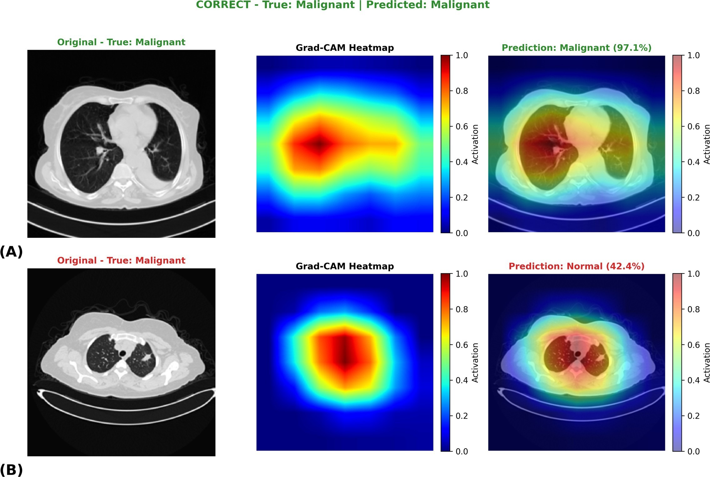
where M is the number of ensemble members and p^(m) is the predicted probability vector of model m. The ensemble procedure, final test evaluation, and Grad-CAM interpretation [28] (Fig. 5) are summarized in Algorithm 3.

Algorithm 3. Ensemble learning, test evaluation, and Grad-CAM interpretation

Require: Trained fusion model fθ*; scaled features r̃; splits Dtr, Dva, Dte
Ensure: Test metrics, confusion matrices, ROC curves, Grad-CAM maps
 1: Train Random Forest (500 trees, balanced class weights) and XGBoost (400 trees, depth 4, learning rate 0.05) on {r̃i}i∈Dtr
 2: Obtain validation probabilities Pdeepva, Prfva, Pgbva
 3: F1best ← −1
 4: for all w = (w1, w2, w3) on a 0.1-step grid with Σi wi = 1 do
 5:     Pensva ← w1Pdeepva + w2Prfva + w3Pgbva
 6:     if macro-F1 of arg max Pensva > F1best then
 7:         update F1best and w* ← w
 8:     end if
 9: end for
10: Penste ← w1*Pdeepte + w2*Prfte + w3*Pgbte
11: for all models m ∈ {Deep, RF, GB, Ensemble} do
12:     Compute accuracy, macro precision, recall, F1, specificity, one-vs-rest ROC-AUC; plot confusion matrix and ROC curves
13: end for
14: Grad-CAM: for the most confident correct and least confident misclassified test patients, back-propagate the predicted-class logit to the last ResNet-18 block
15:     αjk ← (1/hw) Σu,v ∂yc/∂Aj,uvk; Lk ← ReLU(Σj αjkAjk); upsample, normalize to [0, 1], and overlay
16: return metrics, figures, w*

3.9Evaluation metrics

Let TP, TN, FP, and FN denote true positives, true negatives, false positives, and false negatives. For multiclass evaluation, metrics are macro-averaged over classes in a one-vs-rest fashion:

The ROC-AUC was computed in a one-vs-rest manner and macro-averaged. Confusion matrices and ROC curves were also generated.

4Results

4.1Overall test performance

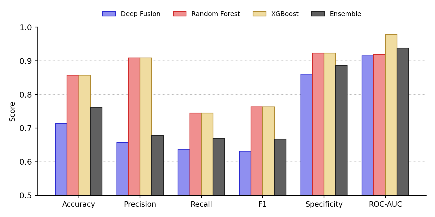
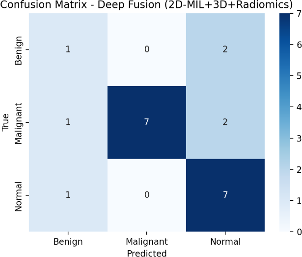
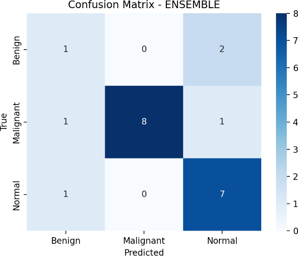
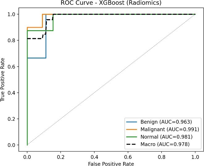
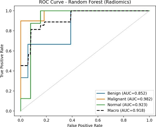
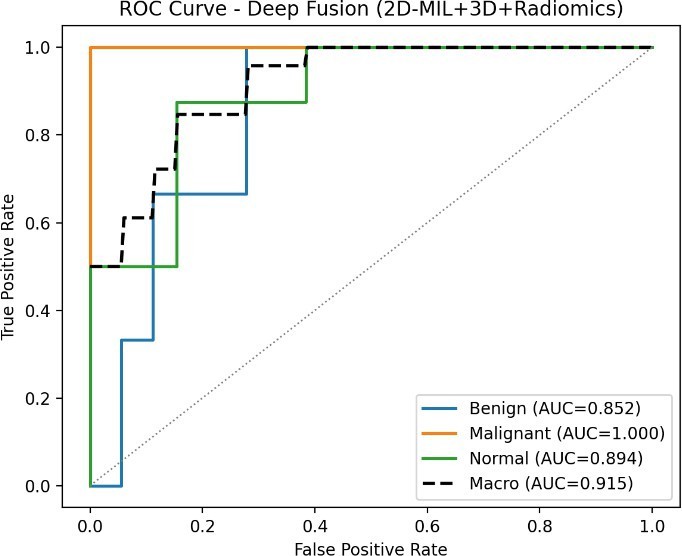
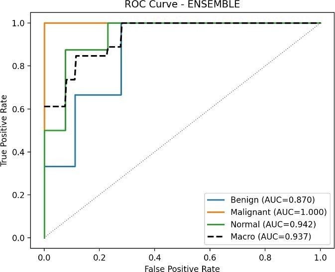
Table 6 and Fig. 2 report the held-out test results of the four models. The two radiomics-based models obtained identical accuracy (0.8571), precision (0.9091), recall (0.7444), F1- score (0.7632), and specificity (0.9231); they differed in ROC-AUC, where XGBoost (0.9782) exceeded Random Forest (0.9189). The deep fusion model (2D-MIL + 3D + Radiomics) achieved an accuracy of 0.7143, an F1-score of 0.6312, and a ROC-AUC of 0.9154. The ensemble improved on the deep fusion model across all metrics (accuracy 0.7619, F1-score 0.6667, ROC-AUC 0.9376) but remained below the radiomics-only models in threshold-dependent metrics.

Model	Acc.	Prec.	Rec.	F1	Spec.	AUC
Deep Fusion	0.7143	0.6566	0.6361	0.6312	0.8604	0.9154
Random Forest	0.8571	0.9091	0.7444	0.7632	0.9231	0.9189
XGBoost	0.8571	0.9091	0.7444	0.7632	0.9231	0.9782
Ensemble	0.7619	0.6778	0.6694	0.6667	0.8860	0.9376

4.2ROC curve and confusion matrix analysis

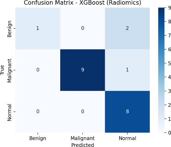
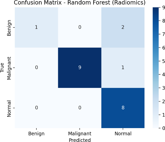
ROC-AUC values were uniformly high (0.9154–0.9782), indicating good class separability for all models (Fig. 4). The gap between the high ROC-AUC and the lower accuracy of the deep fusion model and ensemble suggests that their predicted probabilities rank cases well but that the default decision threshold is suboptimal for some classes. The confusion matrices are shown in Fig. 3.

4.2.1Mathematical solution from the XGBoost (Radiomics) confusion matrix

The numerical results of the proposed XGBoost (Radiomics) model can be verified directly from its test-set confusion matrix in Fig. 3(a). Ordering the classes as Benign (B), Malignant (M), and Normal (N), the confusion matrix is

Here, the rows correspond to the true class labels and the columns correspond to the predicted class labels. The total number of test samples is

Because this is a three-class problem, the metrics are computed for each class in a one-vs-rest manner. For a class c, the outcomes are defined from C as

Applying (14) to (12) gives

For example, for the Normal class, the false positive value of 3 indicates that 3 non-Normal samples (2 Benign and 1 Malignant) were incorrectly classified as Normal, whereas the false negative value of 0 indicates that no Normal sample was missed. Similarly, for the Benign class, the false negative value of 2 indicates that 2 Benign samples were incorrectly classified as Normal.

Overall accuracy. The classification accuracy is the ratio of correctly classified samples (the diagonal of C) to the total number of samples:

Benign class (one-vs-rest). Using TP = 1, FP = 0, FN = 2, and TN = 18:

Malignant class (one-vs-rest). Using TP = 9, FP = 0, FN = 1, and TN = 11:

Normal class (one-vs-rest). Using TP = 8, FP = 3, FN = 0, and TN = 10:

Macro-averaged metrics. The overall metrics reported in Table 6 are obtained by averaging the three class-wise values:

The class-wise counts and metrics are summarized in Table 7. The macro-averaged values (accuracy 0.8571, precision 0.9091, recall 0.7444, specificity 0.9231, and F1-score 0.7632) are identical to the XGBoost (Radiomics) row of Table 6, which confirms that the reported results are consistent with the confusion matrix. The calculation also shows that the lower macro-recall is mainly caused by the Benign class, for which two of the three samples were predicted as Normal, whereas the Malignant and Normal classes were detected with recalls of 0.9000 and 1.0000, respectively.

Class	TP	FP	FN	TN	Prec.	Rec.	Spec.	F1
Benign	1	0	2	18	1.0000	0.3333	1.0000	0.5000
Malignant	9	0	1	11	1.0000	0.9000	1.0000	0.9474
Normal	8	3	0	10	0.7273	1.0000	0.7692	0.8421
Macro avg.	–	–	–	–	0.9091	0.7444	0.9231	0.7632

4.3Comparison with prior work

Table 8 places our results alongside representative published results. Direct comparison should be made with caution because datasets, class definitions, validation protocols, and metrics differ across studies.

Study	Task / Method	AUC	Acc.
Huang et al. [9]	MPLC vs. IPM, CT radiomics	0.889	–
Chen et al. [10]	MPLC vs. IPM, pair relation (training)	0.983	–
Liufu et al. [14]	3-class, MambaOut-Kobe (5-fold CV, image level)	0.946	0.829
Proposed	Test set	0.9782	0.8571

5Discussion

The principal finding is that radiomics-based tree models outperformed the deep fusion network and the ensemble on every threshold-dependent metric, and XGBoost also achieved the highest ROC-AUC. This is consistent with the well-known behavior of deep networks on small cohorts, where a high-capacity model with 2D, 3D, and radiomic branches is prone to overfitting, whereas regularized tree ensembles operating on compact, engineered features are more stable [24], [25]. The ensemble improved over the deep fusion model alone, indicating that combining complementary models is beneficial. However, because the ensemble includes the weaker deep model, its performance fell below that of the radiomics-only models; weighted voting or stacking, with weights chosen on the validation set, may recover this gap.

Compared with prior work, our patient-level design avoids the image-level splitting limitation acknowledged by earlier slice-based studies [14]. The strong ROC-AUC of the radiomics models is in line with the performance of CT radiomics reported for MPLC/IPM differentiation [9], [10].

6Limitations

The main limitation of this study is the relatively small dataset of 1,097 CT images, with an imbalanced distribution among normal, benign, and malignant classes, which may limit the generalizability of the proposed framework. The deep-fusion model also involves multiple high-capacity branches (2D-MIL, 3D, and radiomics), which can be prone to overfitting on limited data. In addition, the experimental evaluation was performed on a single dataset, and therefore the robustness of the models across different institutions, scanners, imaging protocols, and patient populations remains uncertain. The ensemble also did not outperform the radiomics-based XGBoost model, indicating that the current soft-voting strategy may require further optimization.

7Conclusion

We presented a patient-level framework combining deep fusion (2D-MIL, 3D, and radiomics), radiomics-based Random Forest and XGBoost, and an ensemble for differentiating multiple primary lung cancers on CT. Radiomics-based models achieved the best results in this cohort, with XGBoost reaching a ROC-AUC of 0.9782 and both tree models attaining an accuracy of 0.8571, while the deep fusion model and ensemble obtained ROC-AUCs of 0.9154 and 0.9376, respectively. These findings support radiomics-driven models as strong baselines for MPLC differentiation and motivate larger multicenter validation.

8Future work

Future work will focus on validating the proposed framework using larger, diverse, and multicenter CT datasets to improve its clinical generalizability. The framework can be further enhanced by incorporating clinical, histopathological, molecular, and PET/CT information alongside CT radiomics. Weighted voting or stacking strategies can also be investigated to improve ensemble performance. Further research may explore advanced segmentation, feature-selection, explainable AI, probability calibration, and prospective clinical validation to develop a more robust and clinically applicable system for differentiating MPLC, intrapulmonary metastasis, and benign pulmonary lesions.

Data Availability

The dataset is available on Kaggle: https://www.kaggle.com/datasets/arnabdutta123/the-iq-othnccd-lung-cancer-dataset

Code Availability

The code is available on Kaggle: https://www.kaggle.com/code/arnabdutta123/final-lungs-detection

Acknowledgments

The author would like to express sincere gratitude to the Department of Computer Science and Engineering, Pailan College of Management and Technology, for providing the academic environment and support necessary to conduct this research. The author also acknowledges the availability of the IQ-OTHNCCD lung cancer dataset and the open-source tools and libraries used for data processing, radiomics extraction, model development, and evaluation. Finally, the author is grateful to all researchers and contributors whose prior work provided valuable foundations for this study on CT-based lung cancer classification.

References

1. [1]Sung H, Ferlay J, Siegel RL, et al. Global cancer statistics 2020: GLOBOCAN estimates of incidence and mortality worldwide for 36 cancers in 185 countries. CA Cancer J. Clin. 2021;71:209–249. https://doi.org/10.3322/caac.21660
2. [2]Wang YL, Wang YG. Current status and prospects of multiple primary lung cancer research. Chin. J. Cancer Prev. Treat. 2019;26(9):670–674.
3. [3]Yuan L, et al. The advancement of predictive diagnosis and molecular mechanism in multiple primary lung cancer. Chin. J. Cancer. 2010;29(5):575–578. https://doi.org/10.5732/cjc.009.10282
4. [4]Li R, Li X, Xue R, et al. Diagnosis and management of multiple primary lung cancer. J. Thorac. Dis. 2024;16(10):6039–6051. https://doi.org/10.21037/jtd-23-1645
5. [5]Wang Z, Wang S, Chang C, et al. Multiple primary lung cancer: Updates and perspectives. Int. J. Cancer. 2024;155(2):193–207. https://doi.org/10.1002/ijc.34994
6. [6]Zhang Z, Zhang Y, Feng A, et al. Multiple primary lung cancer: Updates of clinical management and challenges. Front. Oncol. 2023;13:1034752. https://doi.org/10.3389/fonc.2023.1034752
7. [7]Kozower BD, Larner JM, Detterbeck FC, Jones DR. Special treatment issues in non-small cell lung cancer: Diagnosis and management of lung cancer, American College of Chest Physicians evidence-based clinical practice guidelines. Chest. 2013;143(5):e369S–e399S. https://doi.org/10.1378/chest.12-2362
8. [8]Girard N, et al. Comprehensive histologic assessment helps to differentiate multiple lung primary nonsmall cell carcinomas from metastases. Am. J. Surg. Pathol. 2009;33:1752–1764. https://doi.org/10.1097/PAS.0b013e3181b8cf03
9. [9]Huang M, Xu Q, Zhou M, Li X, Lv W, Zhou C, et al. Distinguishing multiple primary lung cancers from intrapulmonary metastasis using CT-based radiomics. Eur. J. Radiol. 2023;160:110671. https://doi.org/10.1016/j.ejrad.2022.110671
10. [10]Chen TF, Yang L, Chen HB, Zhou ZG, Wu ZT, Luo HH, et al. A pairwise radiomics algorithm–lesion pair relation estimation model for distinguishing multiple primary lung cancer from intrapulmonary metastasis. Precis. Clin. Med. 2023;6(4):pbad029. https://doi.org/10.1093/pcmedi/pbad029
11. [11]Astaraki M, Yang G, Zakko Y, Toma-Dasu I, Smedby I, Wang C. A comparative study of radiomics and deep-learning based methods for pulmonary nodule malignancy prediction in low dose CT images. Front. Oncol. 2021;11:737368. https://doi.org/10.3389/fonc.2021.737368
12. [12]Suh YJ, Lee HJ, Sung PS, Kim MS, Lee JG, Park S, et al. A novel algorithm to differentiate between multiple primary lung cancers and intrapulmonary metastasis in multiple lung cancers with multiple pulmonary sites of involvement. J. Thorac. Oncol. 2020;15(2):203–215. https://doi.org/10.1016/j.jtho.2019.09.221
13. [13]Shao L, Wang XD, Wu PY, Zhang JQ, Liu LX, Wu CL, et al. A comprehensive algorithm to distinguish between MPLC and IPM in multiple lung tumors patients. Ann. Transl. Med. 2020;8(18):1137. https://doi.org/10.21037/atm-20-5505
14. [14]Liufu Y, Su R, Wen Y, Guan Y, Mahmoud MA. A CT-based deep learning approach to differentiate multiple primary lung cancers, metastases, and benign nodules. BMC Cancer. 2026;26:177. https://doi.org/10.1186/s12885-025-15501-1
15. [15]Gayap HT, Akhloufi MA. Deep machine learning for medical diagnosis, application to lung cancer detection: A review. BioMedInformatics. 2024;4(1):236–284. https://doi.org/10.3390/biomedinformatics4010015
16. [16]Atmakuru A, Chakraborty S, Faust O, Salvi M, Barua PD, Molinari F, et al. Deep learning in radiology for lung cancer diagnostics: A systematic review of classification, segmentation, and predictive modeling techniques. Expert Syst. Appl. 2024;255:124665. https://doi.org/10.1016/j.eswa.2024.124665
17. [17]He K, Zhang X, Ren S, Sun J. Deep residual learning for image recognition. In: Proc. IEEE Conf. Comput. Vis. Pattern Recognit. (CVPR). 2016. p. 770–778. https://doi.org/10.1109/CVPR.2016.90
18. [18]Huang G, Liu Z, van der Maaten L, Weinberger KQ. Densely connected convolutional networks. In: Proc. IEEE Conf. Comput. Vis. Pattern Recognit. (CVPR). 2017. p. 4700–4708. https://doi.org/10.1109/CVPR.2017.243
19. [19]Tan M, Le Q. EfficientNet: Rethinking model scaling for convolutional neural networks. In: Proc. Int. Conf. Mach. Learn. (ICML). 2019. p. 6105–6114.
20. [20]Dosovitskiy A, et al. An image is worth 16×16 words: Transformers for image recognition at scale. arXiv preprint arXiv:2010.11929. 2020. https://doi.org/10.48550/arXiv.2010.11929
21. [21]Liu Z, Hu H, Lin Y, Yao Z, Xie Z, Wei Y, et al. Swin Transformer V2: Scaling up capacity and resolution. In: Proc. IEEE/CVF Conf. Comput. Vis. Pattern Recognit. (CVPR). 2022. p. 12009–12019. https://doi.org/10.1109/CVPR52688.2022.01170
22. [22]Yu W, Wang X. MambaOut: Do we really need Mamba for vision? In: Proc. IEEE/CVF Conf. Comput. Vis. Pattern Recognit. (CVPR). 2025. p. 4484–4496. https://doi.org/10.1109/CVPR52734.2025.00423
23. [23]Ilse M, Tomczak JM, Welling M. Attention-based deep multiple instance learning. In: Proc. Int. Conf. Mach. Learn. (ICML). 2018. p. 2127–2136. https://doi.org/10.48550/arXiv.1802.04712
24. [24]Breiman L. Random forests. Mach. Learn. 2001;45(1):5–32. https://doi.org/10.1023/A:1010933404324
25. [25]Chen T, Guestrin C. XGBoost: A scalable tree boosting system. In: Proc. 22nd ACM SIGKDD Int. Conf. Knowl. Discov. Data Min. 2016. p. 785–794. https://doi.org/10.1145/2939672.2939785
26. [26]van Griethuysen JJM, Fedorov A, Parmar C, et al. Computational radiomics system to decode the radiographic phenotype. Cancer Res. 2017;77(21):e104–e107. https://doi.org/10.1158/0008-5472.CAN-170339
27. [27]Vickers AJ, Elkin EB. Decision curve analysis: A novel method for evaluating prediction models. Med. Decis. Making. 2006;26(6):565–574. https://doi.org/10.1177/0272989X06295361
28. [28]Selvaraju RR, Cogswell A, Das A, Vedantam R, Parikh D, Batra D. Grad-CAM: Visual explanations from deep networks via gradient-based localization. Int. J. Comput. Vis. 2020;128(2):336–359. https://doi.org/10.1007/s11263-019-01228-7