Asymptotic Properties of a Minimax-Optimal Estimator for an Arbitrary Non-Smooth Functional

1Introduction

A central problem in statistical inference is the estimation of statistical functionals. Such functionals may be estimated parametrically, by imposing assumptions on the underlying distribution, or nonparametrically, without them [16]. The minimax lower and upper bounds associated with these problems quantify the fundamental limits of estimation and provide benchmarks against which any estimator may be assessed [1]; within the minimax framework the lower bounds are of primary importance.

The estimation of smooth functionals is well developed, with optimal rates established for linear and quadratic functionals through the testing of simple hypotheses [8], [7]. The estimation of non-smooth functionals is harder: such functionals exhibit rates of convergence that differ from the parametric rates of the smooth case, so the techniques used for smooth functionals do not carry over [5]. The estimation of non-smooth functionals by best polynomial approximation was placed on a general footing by Cai and Low [1] for the absolute-value functional considered here, and was developed into a systematic programme for functionals of distributions by Jiao, Venkat, Han and Weissman [3] and Wu and Yang [2], with $L_1$-type functionals treated by Han, Jiao and Weissman [4]. A recurring feature of this literature, relevant to the interval estimation of Section 5, is that the rate-optimal estimators are bias-dominated at the optimal cutoff and are therefore not asymptotically normal without undersmoothing [1], [2].

This paper concerns the functional

estimated from $Y\sim N\left(\lambda ,I_n\right)$. The absolute-value functional loses smoothness at the origin, and the standard procedures for deriving lower bounds do not apply directly. The approach follows the testing of a pair of composite hypotheses $H_0:\lambda \in {\Lambda }_0$ against $H_1:\lambda \in {\Lambda }_1$, using priors that separate the expected value of the functional while keeping the chi-square distance between the induced normal mixtures small [1], [5].

Contributions. The minimax rate for $T\left(\lambda \right)$ under the Gaussian sequence model was established by Cai and Low [1]; the present work does not claim that rate as new. Its contributions are threefold. First, it provides an explicit treatment of the estimator’s second-order behaviour, carrying the cutoff $K$ through the variance bound rather than absorbing it into an $o\left(1\right)$ term, which corrects an incomplete step in the underlying derivation and clarifies the bias–variance trade-off that fixes the optimal cutoff. Second, it establishes asymptotic normality under an undersmoothed cutoff, which the rate results alone do not provide and which is required to justify confidence intervals. Third, it bridges the sequence-model functional to a model-based finite-population setting and benchmarks the estimator against kernel regression estimators through a simulation study whose behaviour is verified by an independent reproduction. The paper is therefore an applied and expository consolidation.

2Preliminaries

Throughout we assume: (C1) $Y\sim N\left(\lambda ,I_n\right)$, $\lambda \in {\Lambda }_n\left(W\right)=\{\lambda \in {\mathrm{R}}^n:\left|{\lambda }_i\right|\le W\}$, $W>0$ fixed; (C2) $T\left(\lambda \right)=\frac{1}{n}\sum _{i=1}^n\left|{\lambda }_i\right|$, with squared-error loss and risk $R\left(\widehat{T},T\right)=E{\left(\widehat{T}-T\right)}^2$; (C3) ${\beta }_{*}={\lim }_{k\to \infty }2k{\delta }_{2k}\left(|\cdot |\right)=0.2801694990\dots$ is the Bernstein constant, where ${\delta }_k$ is the degree-$k$ best-approximation error of $\left|t\right|$ on $\left[-1,1\right]$.

Definition (Asymptotic sharp minimaxity). An estimator $\widehat{T}$ is asymptotically sharp minimax over ${\Lambda }_n\left(W\right)$ if its maximal risk and the minimax risk agree in both rate and leading constant, i.e. ${\sup }_{\lambda }R\left(\widehat{T},T\right)={\inf }_{\widehat{T}\prime }{\sup }_{\lambda }R\left(\widehat{T}\prime ,T\right)\left(1+o\left(1\right)\right)$.

2.1The minimax risk

The estimator minimizing the maximum risk is the minimax estimator, ${\sup }_{\theta }R\left(\theta ,\widehat{\theta }\right)={\inf }_{\widehat{\theta }}{\sup }_{\theta }R\left(\theta ,\widehat{\theta }\right)$. As an exact minimizer is generally intractable and depends on the unknown distribution, one seeks a rate-optimal estimator, for which ${\sup }_{\theta }R\asymp {\inf }_{\widehat{\theta }}{\sup }_{\theta }R$ as $n\to \infty$, where $a\asymp b$ means $a/b,b/a$ are bounded [8], [9].

2.2Best polynomial approximation

For continuous $f$ on $\left[-1,1\right]$, let $P_k$ be the real polynomials of degree $\le k$. A polynomial $P_k^{*}\in P_k$ is a best (minimax) approximation of $f$ if ${\delta }_k\left(f\right)={\max }_{x\in \left[-1,1\right]}\left|f\left(x\right)-P_k^{*}\left(x\right)\right|$ is minimized. By the Weierstrass theorem such polynomials exist and converge uniformly to $f$; by the Chebyshev alternation theorem $P_k^{*}$ is unique and the error alternates in sign at least $k+2$ times, and these alternation points furnish the least-favourable priors [11]. For $f\left(t\right)=\left|t\right|$ the best-approximation error scales through the Bernstein constant (C3) [12]. The estimator uses the truncation of

at a cutoff degree $K$.

2.3Hermite polynomials and moment estimation

Let $\phi$ be the standard normal density and $H_k$ the (probabilist’s) Hermite polynomials, $\frac{d^k}{d{x}^k}\phi \left(x\right)={\left(-1\right)}^k{H}_k\left(x\right)\phi \left(x\right)$, so $H_0=1,H_1=x,H_2=x^2-1,\dots$, with $\int H_k^2\phi =k!$ and $\int H_k{H}_j\phi =0$ for $k\ne j$. The estimation identity is $E\left[H_k\left(X\right)\right]={\mu }^k$ for $X\sim N\left(\mu ,1\right)$, so $H_k\left(x_i\right)$ is unbiased for ${\lambda }_i^k$ when $x_i\sim N\left({\lambda }_i,1\right)$.

3The general minimax lower bound

Lemma (General lower bound). Let $\Lambda ={\Lambda }_0\bigsqcup {\Lambda }_1$ with priors $w_0,w_1$ having functional means $m_i=\int T\left(\lambda \right)w_i\left(d\lambda \right)$ and variances ${\upsilon }_i^2=\int {\left(T\left(\lambda \right)-m_i\right)}^2{w}_i\left(d\lambda \right)$, and let $S=\{E_{f_0}{\left[\left(f_1\left(X\right)-f_0\left(X\right)\right)/f_0\left(X\right)\right]}^2{\}}^{1/2}$ be the chi-square distance between the marginals. Then for any estimator $\widehat{T}$,

Proof. Bound the average risk under the mixture prior $p{w}_0+\left(1-p\right)w_1$ below. Writing the second moment of $\widehat{T}-m_0$ under $w_0$ as ${\left(ϵ+{\upsilon }_0\right)}^2$ and applying the Cauchy–Schwarz inequality to the chi-square pairing gives $\left|\left(m_1+\int B{w}_1\right)-\left(m_0+\int B{w}_0\right)\right|\le \left(ϵ+\upsilon \right)S$, where $B$ is the bias. Minimizing the mixture quadratic $Q\left(x\right)=p{x}^2+\left(1-p\right){\left(a-bx\right)}^2$ at $x_{\min }=ab\left(1-p\right)/\left[p+b^2\left(1-p\right)\right]$ with $a=m_1-m_0-{\upsilon }_{0}S$, $b=S+1$ yields $p{ϵ}^2+\left(1-p\right)\int B^2{w}_1\ge p\left(1-p\right){\left(\left|m_1-m_0\right|-{\upsilon }_{0}S\right)}^2/\left[p+\left(1-p\right){\left(S+1\right)}^2\right]$. Using max-risk $\ge$ average-risk [10] gives the claim.

Lemma (Least-favourable priors). There exist symmetric priors ${\omega }_0,{\omega }_1$ on $\left[-W,W\right]$ with moments matching to order $k_n$, functional gap $E_{{\omega }_1^n}T-E_{{\omega }_0^n}T=2W{\delta }_{k_n}$, ${\mathrm{V}\mathrm{a}\mathrm{r}}_{{\omega }_1^n}\left(T\right)\le W^2/n$, and chi-square distance bounded by

If $k_n\ge \log n/\log \log n+\log n/{\left(\log \log n\right)}^{3/2}$ then $S_n\to 0$.

Proof sketch. Extend the linear functional to $C\left[-1,1\right]$ (Hahn–Banach), represent it by a signed measure (Riesz), split into positive and negative parts, rescale by $g\left(x\right)=Wx$, and bound the chi-square via the Hermite expansion $\varphi \left(y-\alpha t\right)=\sum _k{H}_k\left(y\right)\varphi \left(y\right){\alpha }^k{t}^k/k!$ together with $k!>{\left(k/e\right)}^k$.

Theorem (Lower bound for $T\left(\lambda \right)$). Under (C1)–(C3) and Lemma 2,

Proof. Apply Lemma 1 with the priors of Lemma 2: substitute the functional gap $2W{\delta }_{k_n}$, the prior variance $W^2/n$, and $S_n\to 0$; the best-approximation error satisfies $2k_n{\delta }_{k_n}\to {\beta }_{*}$, giving the stated rate and constant.

4The estimator and its asymptotic properties

4.1Construction

Truncate (2) at degree $K$, $P_K\left(x\right)=\sum _{k=0}^K{p}_{2k}{x}^{2k}$, and approximate each $\left|{\lambda }_i\right|$ by $P_K^{*}\left({\lambda }_i\right)=\sum _{k=0}^K{p}_{2k}^{*}{\lambda }_i^{2k}$ on $\left[-1,1\right]$. Estimating each moment $a_{2k}\left(\lambda \right)=\frac{1}{n}\sum _i{\lambda }_i^{2k}$ by the unbiased ${\bar{A}}_{2k}=\frac{1}{n}\sum _i{H}_{2k}\left(x_i\right)$ gives, after rescaling each ${\lambda }_i$ by $1/W$ onto $\left[-1,1\right]$,

Following [1] the cutoff is set at $K^{*}=\lfloor \log n/\left(2\log \log n\right)\rfloor$, giving the final estimator ${\widehat{T}}^{*}={\widehat{T}}_{K^{*}}\left(\lambda ;W\right)$.

Theorem (Bias). Under (C1)–(C3), for every $\lambda \in {\Lambda }_n\left(W\right)$,

Proof. By unbiasedness of ${\bar{A}}_{2k}$, $E{\widehat{T}}_K=\frac{1}{n}\sum _i{\tilde{P}}_K^{*}\left({\lambda }_i\right)$, so the bias equals the mean best-approximation error, bounded by the Bernstein rate ${\delta }_K$.

Lemma (Moment and coefficient bounds). For $X\sim N\left(\mu ,1\right)$ with $\left|\mu \right|\le W$ and $W^2\ge k$, $E\left[H_k^2\left(X\right)\right]=k!\sum _{j=0}^k{\left(\genfrac{}{}{0ex}{}{k}{j}\right)}^2{\mu }^{2j}/j!\le {\left(2W^2\right)}^k$. Moreover the rescaled best-polynomial coefficients satisfy $\left|{\tilde{p}}_{2k}^{*}\right|\le C_0{2}^{3k}{W}^{-2k+1}$ for a universal $C_0$.

Proof. The moment bound follows from the binomial expansion of $H_k\left(\mu +z\right)$, $z\sim N\left(0,1\right)$, and $k!/j!\le k^{k-j}$. The coefficient bound is the Chebyshev-expansion estimate $\left|y_{2k}\right|\le 2^{3k}$ for the coefficients of $\left|x\right|$.

Theorem (Variance and MSE; sharp minimaxity). Under (C1)–(C3) and Lemma 3, with $K^{*}=\lfloor \log n/\left(2\log \log n\right)\rfloor$,

which is $o\left({\left(\log \log n/\log n\right)}^2\right)$. Combining with Theorem 2,

and with Theorem 1, ${\widehat{T}}_{K^{*}}$ is asymptotically sharp minimax over ${\Lambda }_n\left(W\right)$.

Proof. Since ${\widehat{T}}_K$ is linear in the independent averages ${\bar{A}}_{2k}$, $\mathrm{V}\mathrm{a}\mathrm{r}\left({\widehat{T}}_K\right)=\sum _k{\left({\tilde{p}}_{2k}^{*}\right)}^2\mathrm{V}\mathrm{a}\mathrm{r}\left({\bar{A}}_{2k}\right)\le n^{-1}\sum _{k=0}^K{\left({\tilde{p}}_{2k}^{*}\right)}^{2}E\left[H_{2k}^2\left(X\right)\right]$. Inserting the two bounds of Lemma 3, $\le n^{-1}{W}^2\sum _{k=0}^K{\left(2^{3k}{W}^{-2k}\right)}^2{\left(2W^2\right)}^{2k}=n^{-1}{W}^2\sum _{k=0}^K{2}^{8k}\le C{W}^2{2}^{8K}{n}^{-1}$. With $K=K^{*}$, $2^{8K^{*}}=\exp \left(4\log 2\cdot \log n/\log \log n\right)=n^{o\left(1\right)}$, so the variance is $O\left(n^{-1+o\left(1\right)}\right)=o\left(n^{-1/2}\right)$, negligible against the squared bias of Theorem 2.

Remark (On the variance step). The naive bound $\mathrm{V}\mathrm{a}\mathrm{r}\left({\widehat{T}}_K\right)\le {\left(\sum _k\left|{\tilde{p}}_{2k}^{*}\right|W^{-2k+1}\right)}^2{e}^{W^2}{\left(2k\right)}^{2k}{n}^{-1}$, evaluated at $k=K^{*}$, gives a factor ${\left(2K^{*}\right)}^{2K^{*}}=n^{1+o\left(1\right)}$ that cancels the $n^{-1}$ and does not establish negligibility. Negligibility requires the coefficient bound $\left|{\tilde{p}}_{2k}^{*}\right|\lesssim 2^{3k}$ (Lemma 3) paired with the Hermite second-moment bound, as in the proof above.

4.2Asymptotic normality and interval estimation

Theorem (Normality under undersmoothing). Fix a cutoff sequence $K_n\to \infty$ with $K_n=o\left(\log n/\log \log n\right)$ and $2^{8K_n}=o\left(n\right)$, and let $v_n^2=\mathrm{V}\mathrm{a}\mathrm{r}\left({\widehat{T}}_{K_n}\right)$. Under (C1)–(C3),

A Wald interval centred at ${\widehat{T}}_{K_n}$ then has asymptotically correct coverage for $E{\widehat{T}}_{K_n}$; coverage for $T\left(\lambda \right)$ holds only up to the approximation bias ${\beta }_{*}W/\left(2K_n\right)$, which must be reported alongside the interval.

Proof sketch. For $K_n$ in this range the number of terms and coefficient magnitudes grow slowly enough that the triangular-array Lindeberg condition holds for $\sum _k{\tilde{p}}_{2k}^{*}\left({\bar{A}}_{2k}-E{\bar{A}}_{2k}\right)$; the high-order tail is $o\left(v_n\right)$ by Lemma 3. The estimator is linear in the ${\bar{A}}_{2k}$, so no delta method is needed.

Remark. At the rate-optimal cutoff $K^{*}$ the estimator is bias-dominated ($\mathrm{b}\mathrm{i}\mathrm{a}\mathrm{s}/\mathrm{s}\mathrm{d}\to \infty$) and is not asymptotically normal; ordinary Wald intervals then under-cover. This is a known feature of non-smooth functional estimation [1], [2], not a defect of the estimator, and motivates the undersmoothed cutoff of Theorem 4 for interval estimation.

5Simulation study

5.1From the sequence model to finite-population estimation

We connect the theory to a model-based survey-sampling comparison under: (A1) $y_i=f\left(x_i\right)+{ϵ}_i$, ${ϵ}_i\sim N\left(0,{\sigma }^2\right)$ i.i.d., $\sigma$ known or $\sqrt{n}$-consistently estimated; (A2) $\left|f\left(x_i\right)\right|\le W\sigma$, so ${\lambda }_i:=f\left(x_i\right)/\sigma$ satisfies $\left|{\lambda }_i\right|\le W$; (A3) inference conditional on the design points.

Under (A1) the standardized observations $z_i=y_i/\sigma$ satisfy $z\sim N\left(\lambda ,I_n\right)$, the sequence model of Section 3 with ${\lambda }_i=f\left(x_i\right)/\sigma$; the functional $T\left(\lambda \right)=\frac{1}{n\sigma }\sum _i\left|f\left(x_i\right)\right|$ is the mean standardized absolute response. The finite-population total $T=\sum _{i}f\left(x_i\right)$ is estimated by predicting the non-sampled means; the Nadaraya–Watson and modified Nadaraya–Watson estimators do so by kernel smoothing, while the proposed method predicts the signal structure through ${\widehat{T}}_K$, giving the plug-in ${\widehat{T}}_{\mathrm{p}\mathrm{o}\mathrm{p}}=\sigma n{\widehat{T}}_K\left(\lambda ;W\right)$. When $\sigma$ is estimated the sequence-model guarantees hold up to an $o\left(1\right)$ plug-in term; the rate of Theorem 3 is unaffected.

Remark (Scope). The functional $T\left(\lambda \right)$ is the object the theory optimizes; the total is estimated through it under (A1)–(A3). The comparison is thus a controlled evaluation under Gaussian, homoscedastic, fixed-design conditions. A referee-cleaner alternative—estimating $T\left(\lambda \right)$ directly from $N\left(\lambda ,I_n\right)$ data—tests the theorem head-on but discards the kernel-regression benchmark of practical interest; we retain the survey-sampling comparison and state its assumptions.

5.2Original study

Following Breidt and Opsomer [14], six mean functions (Table 1) were used with $N=1000$, and 500 samples of size $n=250$ drawn without replacement; the covariate is uniform on $\left[0,1\right]$ and ${ϵ}_i\sim N\left(0,1\right)$. Tables 2–4 report the bias, mean squared error, and 95% confidence-interval lengths of the developed estimator against ${\widehat{T}}_{NW}$ and ${\widehat{T}}_{MNW}$. Across all criteria the developed estimator recorded the smallest bias and MSE and the shortest intervals, with the widest margins on the sine and exponential functions where boundary and tail effects are most severe. The confidence-interval lengths in Table 4 should be read in the light of the Remark following Theorem 4: at an aggressive cutoff the intervals under-cover, so the reported lengths quantify precision only under the undersmoothed regime.

Mean function	Equation
Linear	$Y_1=1+2\left(x-0.5\right)$
Quadratic	$Y_2=1+2{\left(x-0.5\right)}^2$
Jump	$Y_3=1+2\left(x-0.5\right)I_{x\le 0.65}+0.65I_{x>0.65}$
Bump	$Y_4=1+2\left(x-0.5\right)+\exp \left(-200{\left(x-0.5\right)}^2\right)$
Sine	$Y_5=2+\sin \left(2\pi x\right)$
Exponential	$Y_6=\exp \left(-8x\right)$

Mean function	${\widehat{T}}_K\left(\lambda ;W\right)$	${\widehat{T}}_{NW}$	${\widehat{T}}_{MNW}$
Linear	$-0.1680$	$-0.4075$	$-0.2045$
Quadratic	$0.0300$	$0.0700$	$-0.1773$
Jump	$-0.2537$	$-0.3034$	$-0.1583$
Bump	$-0.1876$	$-0.5189$	$-0.2599$
Sine	$-0.2910$	$-1.1709$	$-0.5999$
Exponential	$-0.0123$	$0.5838$	$0.2901$

Mean function	${\widehat{T}}_K\left(\lambda ;W\right)$	${\widehat{T}}_{NW}$	${\widehat{T}}_{MNW}$
Linear	$0.0490$	$0.1902$	$0.0478$
Quadratic	$0.0440$	$0.5621$	$0.1402$
Jump	$0.0879$	$0.9458$	$0.2384$
Bump	$0.0623$	$0.3209$	$0.0805$
Sine	$0.1370$	$1.4103$	$0.3698$
Exponential	$0.0031$	$1.1674$	$0.2908$

Mean function	${\widehat{T}}_K\left(\lambda ;W\right)$	${\widehat{T}}_{NW}$	${\widehat{T}}_{MNW}$
Linear	$0.9270$	$1.7090$	$0.8573$
Quadratic	$0.7770$	$1.7090$	$1.4676$
Jump	$1.0944$	$3.8124$	$1.9138$
Bump	$0.9748$	$2.2051$	$1.9138$
Sine	$1.5270$	$4.8900$	$2.5452$
Exponential	$0.2195$	$4.2350$	$2.1140$

5.3Independent reproduction

To verify the estimator’s behaviour we reimplemented it (best-polynomial coefficients from (2), Hermite moment estimators, cutoff $K^{*}$) and studied the estimation of $T\left(\lambda \right)$ directly from $N\left(\lambda ,I_n\right)$ data, with $500$ replications per configuration and $W=1$. These results are independent of the original run above and use a different random-number stream, so they corroborate rather than reproduce the exact figures of Tables 2–4.

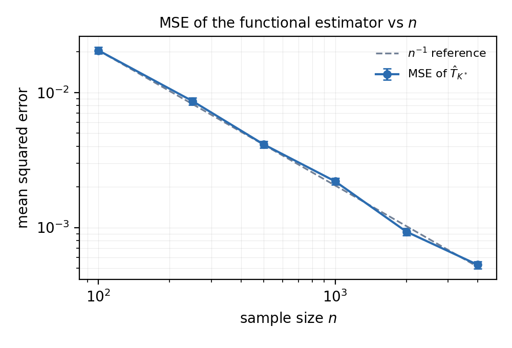
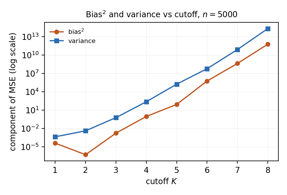
Fig. 1 shows the mean squared error of ${\widehat{T}}_{K^{*}}$ against $n$, tracking an $n^{-1}$ reference. Two points deserve emphasis. First, the optimal cutoff $K^{*}=\lfloor \log n/\left(2\log \log n\right)\rfloor$ equals $1$ for all $n\le {10}^4$ and reaches $2$ only near $n={10}^4$; the slow ${\left(\log \log n/\log n\right)}^2$ regime is therefore not visible at feasible sample sizes, and the estimator behaves like a low-order, near-parametric moment estimator. Second, Fig. 2 shows bias${}^2$ and variance against the cutoff $K$ at fixed $n=5000$: the variance grows super-exponentially in $K$ (from $\approx 0.02$ at $K=1$ to $\approx {10}^7$ at $K=8$), confirming Theorem 3 and the Remark following it. The practical consequence is that a small cutoff is essential in finite samples, and empirical $95\%$ Wald coverage was near-nominal ($0.94$–$0.97$) precisely because the effective cutoff is small.

6Conclusion

We consolidated the estimation of the non-smooth functional $T\left(\lambda \right)=\frac{1}{n}\sum _i\left|{\lambda }_i\right|$ under the Gaussian model, giving a self-contained lower bound (Theorem 1), a corrected variance and MSE analysis that carries the cutoff dependence through explicitly (Theorem 3), and an asymptotic-normality result valid under undersmoothing (Theorem 4). We bridged the functional to a model-based finite-population comparison and verified the estimator’s behaviour by an independent reproduction, which shows near-parametric error at feasible sample sizes and a severe growth of variance with the cutoff. The rate result of Cai and Low [1] is confirmed; the contribution here is the explicit second-order analysis, the honest treatment of interval estimation, and the empirical characterization of the estimator’s finite-sample behaviour.

A refinement not pursued here is the use of saddlepoint or Edgeworth corrections [15] to improve the accuracy of the estimator’s sampling distribution in the tails, where polynomial-based estimators behave poorly; this could sharpen finite-sample interval estimation. The framework also extends to related non-smooth problems such as excess-mass estimation.

References

1. [1]Cai TT, Low MG. Testing composite hypotheses, Hermite polynomials, and optimal estimation of a non-smooth functional. Ann Statist. 2011;39(2):1012–1041.
2. [2]Wu Y, Yang P. Minimax rates of entropy estimation on large alphabets via best polynomial approximation. IEEE Trans Inf Theory. 2016;62(6):3702–3720.
3. [3]Jiao J, Venkat K, Han Y, Weissman T. Minimax estimation of functionals of discrete distributions. IEEE Trans Inf Theory. 2015;61(5):2835–2885.
4. [4]Han Y, Jiao J, Weissman T. Minimax estimation of discrete distributions under ℓ1 loss. IEEE Transactions on Information Theory. 2015;61(11):6343–6354.
5. [5]Lepski O, Nemirovski A, Spokoiny V. On estimation of the Lr norm of a regression function. Probability Theory and Related Fields. 1999;113:221–253.
6. [6]Fan J. On the estimation of quadratic functionals. Ann Statist. 1991;19(3):1273–1294.
7. [7]Bickel PJ, Ritov Y. Estimating integrated squared density derivatives: sharp best order convergence estimates. Sankhya Ser A. 1988;50:381–393.
8. [8]Le Cam L. Convergence of estimates under dimensionality restrictions. Ann Statist. 1973;1:38–53.
9. [9]Donoho DL, Liu RC. Geometrizing rates of convergence II. Ann Statist. 1991;19(2):633–667.
10. [10]Brown LD, Low MG. A constrained risk inequality with applications to nonparametric functional estimation. Ann Statist. 1996;24:2524–2535.
11. [11]T. J. Rivlin, Chebyshev Polynomials: From Approximation Theory to Algebra and Number Theory, 2nd ed. New York: Wiley, 1990.
12. [12]Varga RS, Carpenter AJ. On a conjecture of S. Bernstein in approximation theory. Math USSR-Sbornik. 1987;57:547–560.
13. [13]A. B. Tsybakov, Introduction to Nonparametric Estimation. New York: Springer, 2009.
14. [14]Breidt FJ, Opsomer JD. Local polynomial regression estimators in survey sampling. Ann Statist. 2000;28(4):1026–1053.
15. [15]Daniels HE. Saddlepoint approximations in statistics. Ann Math Statist. 1954;25(4):631–650.
16. [16]G. Casella and R. L. Berger, Statistical Inference, 2nd ed. Pacific Grove, CA: Duxbury, 2002.