Beyond Leaf Images: A Personalized Multimodal Temporal AI Framework for Pre-Symptomatic Plant Health Monitoring and Disease-Risk Early Warning

1Introduction

Crop production now faces constraints that earlier systems barely felt. Water is scarce, labour costs keep climbing and weather is harder to predict from one season to the next, so decisions have to be more targeted. That pressure has pushed precision agriculture toward continuous sensing and analysis. Artificial intelligence (AI) can turn large streams of observations into usable information for a field zone, a greenhouse bench or a single plant [1]. Disease management is among its busiest applications: losses can build quickly, and many symptoms are hard to score consistently by hand.

Most plant disease systems still follow one familiar sequence: capture an image, extract visual features and predict a class. Convolutional neural networks (CNNs), transfer learning, object detection, image segmentation, vision transformers and lightweight networks have all sharpened this pipeline [2–6]. None of that should be dismissed. A good RGB image shows a lesion directly, a person can inspect it, and labelling it often costs less than labelling sensor-based measurements. For many practical tasks, image analysis is the easiest place to start.

The difficulty is timing. A visible lesion is the end result of changes that began earlier. Transpiration, tissue temperature, pigment behaviour, leaf structure and electrical activity can all shift while the plant still looks normal to a grower [7]. Work on asymptomatic detection has grown, including hyperspectral measurements paired with machine learning [8], yet the literature still lacks a shared, time-based measure of earliness. A claim that a system detects disease early is hard to interpret when one study means a few hours before visible change and another means several days before laboratory confirmation.

Unusual appearance also does not equal disease. Wilting may reflect water shortage, chlorosis may come from a nutrient imbalance, and leaf damage may follow heat, chemicals or mechanical injury. A model trained to choose only among disease classes can be forced to name a disease for an observation that something else caused [5, 6, 9, 10]. Such a model may look precise on a test set and still be difficult to use in a real crop environment.

Plant health is therefore better treated as a trajectory than as a collection of unrelated photographs. Environmental exposure shifts through the day, soil moisture rises and falls with irrigation, leaf temperature responds to radiation, wind and transpiration, and plant electrical signals vary with stimulation. A single photograph carries no memory of any of this; a time-aligned record does.

PlantPulse is built on that idea and asks a different operational question: has this particular plant begun to behave differently from its own recent pattern, and does the surrounding evidence make disease a plausible explanation? The word particular matters. Two plants side by side may receive the same irrigation and air temperature yet respond differently. A population average can hide that difference; a personalized reference can expose it.

Personalization also changes the purpose of anomaly detection. At the first stage the system does not need to know the disease, only whether something has changed. A later risk layer asks whether the change fits normal growth, environmental stress or disease risk. If the evidence is weak, the system returns an insufficient evidence state instead of a forced label.

The paper makes four contributions. First, it brings together the sensing channels that can carry information before strong visual symptoms appear and discusses the limits of each. Second, it proposes a layered architecture that runs from sensing and synchronization to uncertainty-aware decision support. Third, it gives a formal representation for personalized temporal modelling, including a standardized deviation measure and a history window. Fourth, it sets out an evaluation strategy that treats lead time, false alarm burden, calibration, robustness and ablation as central outcomes. The paper does not assume that more sensors or a larger network must be better; it sets out to measure when additional information helps and when it does not.

The paper proceeds as follows. It first reviews image-based recognition and its limits for early warning, then surveys the candidate sensing channels. The research gap and design principles are stated next, followed by a description of the seven-layer PlantPulse framework and its data representation and models. An evaluation protocol is then defined, after which explainability, reproducibility and deployment are discussed. The paper closes with open challenges, future directions and conclusions.

2Image-based plant disease recognition and its limits

2.1State of the art

Image-based recognition is the most established part of plant disease AI. Early work showed that CNNs could classify disease categories from leaf images with high benchmark accuracy [2, 3]. Researchers then moved to pre-trained networks such as ResNet, DenseNet, EfficientNet and MobileNet, usually adapted to crop-specific datasets. Newer systems add vision transformers, CNN-transformer hybrids, lesion detectors, segmentation models and compressed networks for mobile or edge use [4–6]. Explanation tools such as Grad-CAM can show which image regions drove a prediction [11].

This progress has clear causes. Cameras cost little compared with most specialist sensing systems, and smartphones already capture images at useful resolution. Image datasets are also easier to annotate than continuous electrical or gas sensor streams, because a labelled image ties directly to an observed condition. These strengths make RGB imaging a practical part of PlantPulse, not an obsolete one.

2.2Why accuracy is not enough

The first issue is dataset bias. Many benchmark collections were built with controlled framing, known lighting, clean backgrounds and predictable acquisition conditions. A model can learn features that correlate with a class without representing the underlying biology; background texture, camera characteristics, illumination or acquisition habits can slip into the decision rule [9, 10]. When the same model is moved to a new field, cultivar, camera or season, performance may drop.

The second issue is confusion between disease and abiotic stress. A yellow leaf is not a diagnosis, and neither is wilting. Necrosis and leaf curling have several possible causes [5, 6, 9, 10]. The appearance can be real while the interpretation is wrong, and the problem sharpens when the model has no access to soil water, recent temperature, leaf wetness or any other context that could support a competing explanation.

The third issue is the snapshot problem. One image captures a state but not a history. It cannot show whether the same leaf was stable yesterday, whether soil moisture dropped after a missed irrigation, or whether leaf temperature has slowly drifted away from air temperature over several days. A temporal record supplies those comparisons and may reveal a change before the camera can show a distinctive lesion.

2.3Implications for PlantPulse

PlantPulse keeps image analysis but changes its place in the workflow. The image becomes one link in a longer chain of evidence: RGB data can confirm visible symptoms, assist expert labelling and serve as an image-only baseline. The framework also leaves room for a fair negative result. If an image-only model matches the full multimodal design for a given crop and environment, that finding is scientifically useful.

3Sensing modalities for pre-symptomatic plant health monitoring

No sensor measures plant health as a single, complete quantity. Each channel observes a different aspect of the plant and its surroundings, and each has weaknesses that can mislead. PlantPulse therefore treats multimodality as a way to compare and combine partial views, not as a guarantee of better prediction. Table 1 summarizes the modalities considered.

3.1Environmental and soil sensing

Air temperature, relative humidity (RH), light, leaf wetness and rainfall describe the background in which plants grow and pathogens develop. Disease forecasting has long used these variables, and environmental records can support machine learning models that estimate disease-favourable periods [12]. Leaf wetness is especially useful for foliar disease studies because surface moisture influences pathogen establishment. Soil moisture and soil temperature add a root-zone view that helps separate water-related stress from other forms of plant change.

The main limitation is indirectness. Environmental variables describe exposure, not how a specific plant responded, and two neighbouring plants can experience the same air temperature yet follow different physiological trajectories. PlantPulse therefore uses environmental data as context. A rise in leaf temperature means one thing when the air is hot and dry and another when it is cool and humid; soil moisture likewise reads differently at different growth stages.

3.2Plant electrophysiology and impedance

Plants generate measurable electrical signals in response to several kinds of stimulation, including wounding, temperature change and shifts in water status [13]. Electrical activity and tissue impedance can be sampled with surface or inserted electrodes. Recent work has paired machine learning with implantable electrophysiological sensors for stress monitoring and has examined plant electrical signals as indicators of environmental conditions [14, 15].

This channel is attractive because it measures a response generated by the plant itself, and it can be sampled far more often than a camera, opening the door to short-lived changes that daily imaging would miss. The practical cost is high. Electrode type, placement, contact quality, plant anatomy, movement and ambient electrical noise all shape the measurement [13–15]. A robust PlantPulse implementation must separate biological variation from acquisition artefacts. The framework does not assume that electrophysiology will outperform other channels; its added value has to be demonstrated through ablation experiments.

3.3Thermal sensing

Leaf temperature reflects the balance between absorbed energy and transpirational cooling, which is why thermal sensing has long been used to study stomatal behaviour and plant water status [16]. Infection can alter transpiration as well. Thermal imaging has revealed local temperature differences in cucumber leaves affected by downy mildew [17], and broader stress studies show that thermal and related optical signals can change before visible damage appears [18].

Thermal readings depend heavily on measurement conditions: air temperature, incoming radiation, wind, humidity, viewing angle, distance and surface emissivity can all shift a value. Leaf temperature taken alone would therefore be an unreliable disease marker. PlantPulse gives more weight to the relationship between leaf or canopy temperature and its surroundings. The leaf-to-air temperature difference, change from the plant baseline and sustained deviation over time carry more context than any single absolute value.

3.4Volatile organic compound sensing

Plants release volatile organic compounds (VOCs), and the emitted mixture can change under pathogen infection and pest attack. Electronic nose systems built from arrays of low-cost gas sensors have been studied as a practical way to capture these changes [19]. The channel is appealing because it provides chemical information that neither an RGB camera nor a conventional temperature sensor can offer.

The difficulty is selectivity. Metal oxide semiconductor (MOS) sensor arrays respond to several gases, and humidity, temperature, airflow and sensor ageing can all alter the apparent signal [19]. A useful VOC system therefore needs baseline tracking, drift correction and environmental compensation. PlantPulse treats VOC sensing as optional and best suited to enclosed or semi-enclosed settings, such as growth chambers and greenhouses, where airflow is easier to control. The goal is to test whether the chemical channel adds information, not to assume that it does.

3.5RGB imaging

RGB images remain an important reference channel. They give direct visual evidence, allow experts to inspect the plant, and make it possible to compare the temporal approach with a familiar image-only baseline. PlantPulse acquires images periodically rather than continuously, since the environmental and physiological channels can be sampled more often. Sparse imaging also prevents the most easily labelled modality from dominating a fusion model for that reason alone.

3.6Digital twins and continuous crop monitoring

Agricultural digital twins maintain a virtual representation of a crop or growing environment and update it as new sensor observations arrive [20–22]. Recent work has combined microclimate sensing with crop growth prediction and has used sensor gateways to track soil and environmental anomalies [20–22]. PlantPulse is close to this direction but narrower in aim. Its central object is the individual plant baseline, and its main outcome is early warning ahead of a reference event. The distinction matters: a digital model of an entire greenhouse can be useful without solving the problem of spotting a subtle trajectory change in one plant.

Modality	What it observes	Typical sampling	Main strength	Main confounders
Environmental	Air temperature, RH, light, leaf wetness	1-15 min	Low cost; context linked to disease-favourable conditions	Indirect; plants may respond differently
Soil	Moisture, temperature, electrical conductivity	5-60 min	Root-zone context and evidence of water stress	Substrate effects and sensor drift
Electrophysiology / impedance	Electrical activity and tissue properties	Sub-second to minutes	Close to plant physiology	Electrode contact, movement, noise, anatomy
Thermal	Leaf or canopy temperature	Minutes to hours	Indicator of transpiration and water status	Radiation, wind, humidity, geometry, emissivity
VOC / gas	Volatile compounds emitted by the plant	1-10 min	Chemical evidence of stress or attack	Cross-sensitivity, humidity, airflow, drift
RGB	Visible appearance	Once to several times per day	Direct symptoms; easy expert inspection	Late signal, lighting, occlusion, background

4Research gap and design principles

4.1Research gap

The reviewed evidence points to four related gaps. The first is the move from snapshots to trajectories. Much plant disease AI still takes the image as its basic unit, yet early warning requires knowing what happened to the plant over time. The second is the lack of a common measure of earliness, since studies of asymptomatic detection do not always report warning time in a form that allows direct comparison [8]. The third is limited knowledge of the information each modality contributes. A multimodal model can show that fusion works without showing that every sensor contributes enough to justify its hardware, calibration and maintenance burden. The fourth is robustness. Real monitoring systems face missing data, failed sensors, shifting environments and uncertain observations, and evaluation should treat these as normal operating conditions rather than exceptional failures.

The components PlantPulse needs already exist as active research areas. Environmental disease forecasting, plant electrophysiology, thermal monitoring, VOC sensing, hyperspectral early detection and digital crop representations have all been studied [7, 8, 11–22]. The proposed contribution is therefore a system formulation: it joins a per-plant temporal reference to multimodal interpretation, explicit uncertainty and an evaluation that treats lead time as a central outcome.

4.2Design principles

• Plant-centred reference. Normality is defined by the plant's own history, adjusted for diurnal effects and growth stage.
• Evidence over forced labelling. Risk and uncertainty are outputs; the system does not demand a class for every anomalous observation.
• Earliness as a measured outcome. Warning lead time is reported together with the false alarm burden and the type of reference event detected.
• Justified complexity. A sensor or model component remains in the final design only if it produces a demonstrable gain on a meaningful metric.
• Graceful degradation. When a modality drops out, the system continues on the remaining channels and lowers its confidence instead of concealing the loss of evidence.

5The PlantPulse framework

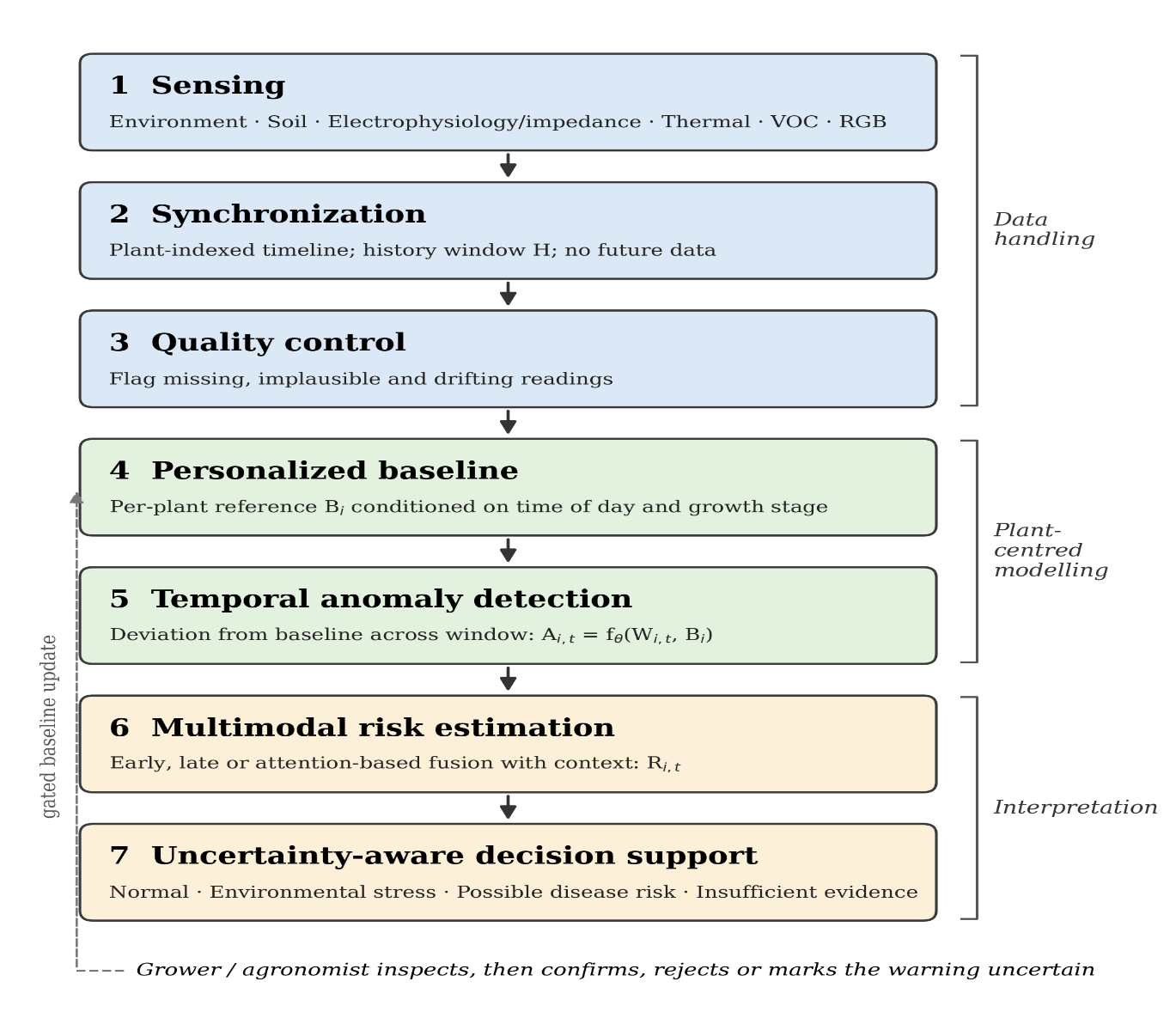
PlantPulse comprises seven connected layers (Figure 1). The first layers turn raw measurements into a clean, plant-indexed record. The middle layers learn what is usual for each plant and flag deviations. The final layers interpret a deviation, estimate uncertainty and present a warning to a human user. The architecture is modular: a simple statistical baseline can be deployed first and replaced by more advanced models as the dataset grows, while the evaluation rules remain fixed.

5.1Sensing layer

A practical minimum configuration starts with air temperature and relative humidity, which are inexpensive and relevant to both plant stress and pathogen-favourable conditions. Soil moisture adds information on root-zone water availability, light intensity helps interpret photosynthetic and thermal changes, and leaf wetness, where feasible, gives a more direct reading of surface moisture. An extended configuration can add electrophysiological or impedance electrodes, a thermal sensor and a small MOS gas sensor array in controlled environments. RGB images are captured at defined intervals rather than continuously. Hardware choices are left open, to be determined by the biological question, the required sampling rate and the deployment setting.

5.2Synchronization

The signals do not arrive at the same rate. Electrical measurements may be recorded many times per second, environmental sensors may log every few minutes, and images may be captured once or twice a day. Every measurement therefore needs at least a timestamp and a plant identifier. To predict at time t, the system builds a history window of length H from the observations available by that time. The window can be summarized using means, medians, variances, extrema, slopes, rates of change, moving averages, frequency-domain features for high-rate signals and deviations from the personal baseline. One rule is simple and critical: future information must never enter a prediction about the past. This must hold throughout feature creation, interpolation, normalization and model training.

5.3Quality control

Quality control is part of the scientific model, not a pre-processing chore. Environmental and soil sensors can produce missing values, impossible values, saturation, abrupt jumps, disconnections and timestamp errors. Electrical channels need checks for electrode contact and movement artefacts. Thermal frames need a valid leaf region and stable acquisition conditions. VOC signals should be corrected for temperature and humidity and checked for baseline drift, and RGB images need screening for blur, exposure problems and framing errors. Observations that fail a check should be flagged rather than deleted, because the rejection rate varies between environments and can itself reveal differences in deployment quality.

5.4Personalized baseline

For each plant i, PlantPulse learns a baseline B_i during a reference period judged to represent healthy behaviour. A basic version uses a rolling mean and standard deviation for each variable, conditioned on time of day. More advanced versions can use probabilistic trajectory models or an autoencoder trained on normal windows. Diurnal cycles must be handled explicitly: a reading that looks unusual at midday may be normal at night, and vice versa. Growth stage matters for the same reason, since a young plant and a mature plant of the same cultivar do not share normal ranges.

5.5Temporal anomaly detection

The framework does not prescribe a single family of models. Classical options include statistical process control, Isolation Forest [23], one-class support vector machines (SVMs) [24], random forests [25] and gradient-boosted trees [26] applied to engineered temporal features. Neural options include long short-term memory (LSTM) networks [27], gated recurrent units (GRUs) [28], temporal convolutional networks (TCNs) [29] and temporal transformer encoders [30]. Each strikes a different balance between data requirements, interpretability, computational cost and the ability to represent long-range dependencies. The history window H is itself a design choice. Short windows respond quickly but can miss slow change, whereas long windows capture gradual drift but can dampen the response to sudden events. H should be selected on validation data only.

5.6Multimodal fusion

PlantPulse compares three fusion strategies [31]. Early fusion concatenates features from the available modalities before the temporal model; it is straightforward, but differences in scale and missing values can become difficult to manage. Late fusion trains one model per modality and combines their outputs, which tolerates missing channels and allows each model to specialize. Attention-based fusion learns time-dependent weights so that the model can shift which channel matters most at different moments; for instance, environmental measurements may supply background conditions while physiological signals gain weight during an unusual episode. Attention is not presumed to be superior and must demonstrate a measurable benefit.

5.7Uncertainty and abstention

A monitoring system should report not only a risk estimate but also how much confidence that estimate deserves. Candidate approaches include deep ensembles, Monte Carlo dropout, conformal methods and post hoc calibration such as temperature scaling [32–34]. The decision layer combines the anomaly score, risk, uncertainty and data quality information into four states: normal, environmental stress, possible disease risk and insufficient evidence (Table 2). The fourth state is essential. When the input is unfamiliar, the sensors are unreliable or the evidence is contradictory, the appropriate response may be to request further observation rather than to invent a disease label.

State	Triggering condition	Example system message
Normal	Behaviour is consistent with the plant baseline and uncertainty is low	No action needed
Environmental stress	Anomaly detected, and environmental evidence offers a plausible non-disease explanation	Check irrigation or microclimate
Possible disease risk	Anomaly detected, and context is compatible with disease development	Inspect plant and consider expert confirmation
Insufficient evidence	High uncertainty, out-of-distribution input or poor sensor quality	Check sensors and continue monitoring

5.8Decision support

PlantPulse is a decision support system. It does not prescribe actions such as a specific chemical treatment. A warning may suggest closer observation, a sensor check or expert inspection, while interpretation remains with growers and specialists, who are better placed to judge whether and how to act. The system should make the evidence easy to examine rather than hide it behind a single score.

6Data representation and model formulation

6.1Plant state and history window

The state of plant i at time t is represented as a set of modality blocks:

where E contains environmental variables, S soil variables, P electrophysiological or impedance features, T thermal features, G gas (VOC) sensor features and V visual (RGB) features. A block may be empty if the corresponding sensor is unavailable at that time. The history window is denoted:

This representation allows the system to handle mixed sampling rates while preserving plant identity and time. In practice, high-rate channels can be summarized before fusion, and lower-rate channels aligned to the prediction time using rules that rely only on information available at that moment.

6.2Personalized deviation

A simple personalized score compares the current value with the value expected for that plant at the same time of day:

Here x is the current measurement, and μ and σ are the baseline mean and standard deviation for plant i. The small constant ε prevents division by zero when the baseline variance is very small. The standardized value places variables with different units on a common scale and is directly interpretable: a large positive or negative value indicates that the current measurement lies far from that plant's normal range at comparable times of day.

Time of day can be represented using cyclical features:

where h is the hour of day. The cyclical encoding prevents midnight from appearing distant from late evening. Growth stage or days after transplanting can be encoded in the same way when those data are available.

6.3Anomaly, risk and uncertainty

A temporal model with parameters θ maps the recent window and the baseline to an anomaly score:

A second model combines the anomaly score with the temporal window and a context vector C containing disease-favourable indicators and data quality flags:

The risk vector R represents at least two interpretations of an unusual episode: abiotic stress and disease risk. The model also returns an uncertainty estimate U, and the decision layer operates on A, R and U. A high anomaly score does not imply disease; its interpretation depends on the surrounding evidence and on whether the system is operating within the space covered by its training data.

6.4Implementing personalization

Three levels of personalization can be compared. Baseline subtraction is the simplest: measurements are standardized against each plant's own reference before entering a shared model. Plant embeddings use a learned vector derived from each plant's history, allowing a common model to condition its behaviour on that representation. Hierarchical models sit between population models and fully separate ones: shared parameters capture patterns common to the monitored group, while plant-specific deviations are estimated separately. A plant with limited history can then borrow information from others without being forced into a single population average.

6.5Cold start and baseline updating

A new plant has no history, which is a practical constraint rather than a minor technical detail. PlantPulse studies should report performance as the baseline period grows (for example, after 1, 3, 7 and 14 days) to establish how much history is needed before personalization helps. The baseline must also adapt as the plant grows, yet unrestricted updating risks baseline contamination: if disease begins and the model continues learning from the abnormal period, it may gradually absorb the disease pattern as normal. One safeguard is gated updating, in which only high-confidence normal observations may modify the baseline. Another is a dual baseline, in which a stable reference is retained while a second baseline adapts slowly to current conditions. Both raw and processed data should be retained so that a later review can distinguish a sensor problem from a modelling problem.

7Experimental methodology and evaluation protocol

An early warning system should be judged on three linked questions: Did it detect a real event? How much warning did it give? What did that warning cost? Accuracy alone cannot answer all three. A useful experiment requires longitudinal data, independent reference events, leakage control and metrics suited to rare-event monitoring. The protocol below is intended for a future empirical study of PlantPulse; it is not a report of results.

7.1Data strategy

A practical study may combine publicly available environmental disease datasets with a smaller longitudinal dataset collected for per-plant modelling. Public datasets support reproducible baseline experiments and show how much predictive information environmental history carries on its own [12]. They cannot address personalization by themselves, however, because personalization requires repeated, reliably time-aligned observations of the same plant.

For the temporal component, a few plants monitored densely across a full growing cycle can be more informative than a very large collection of unrelated leaf photographs. The final sample size should follow from expected event frequency, statistical power and feasibility of collection. Because disease is usually a rare event, sample size should be counted in events and plant histories rather than raw sensor records.

The monitoring period should record observations without assuming that every anomaly is disease, so that the dataset contains normal variation, environmental stress, sensor faults and genuine disease episodes. Where controlled stress or inoculation experiments are used, they should follow approved agricultural, biosafety and institutional procedures under plant pathology supervision. The aim is not artificial complexity but independently established reference events.

7.2Ground truth

Sensor predictions cannot validate themselves. Reference events must be established independently, through expert inspection, documented agronomic records or laboratory confirmation. Four labels are proposed. Normal means no abnormality was observed. Abiotic stress means an established environmental or physiological stressor with no evidence of pathogen involvement. Suspected disease means that expert inspection indicates disease but confirmation is incomplete. Confirmed disease means that independent diagnostic evidence exists.

Each event is assigned the timestamp of the earliest independent observation used as its reference. This matters because the true biological onset of infection is rarely observed directly: a symptom may appear after infection, and laboratory confirmation may come later still. Stating the reference event makes lead time transparent and comparable across studies.

7.3Defining lead time

Let T_w be the time of the first reliable warning and T_r the time of the independently established reference event, such as the first visible abnormality or laboratory confirmation. Lead time is defined as:

A positive L means the warning preceded the reference event; a negative value means it came afterwards. A warning not followed by a verified event within a predefined horizon counts as a false alarm. Lead time should be reported as a distribution, with the median, interquartile range and per-event values. A single mean can conceal the difference between a system that warns early and consistently and one that succeeds only on a few easy cases.

7.4Data splitting and leakage control

Random row-level splitting is inappropriate for longitudinal data, because adjacent measurements from the same plant can fall into both training and test sets, making the task appear easier than it would be in deployment. PlantPulse should use at least three forms of separation. Plant-wise splitting keeps some plants entirely outside training, measuring generalization to new individuals. Time-wise splitting trains on earlier periods and tests on later ones, mirroring deployment. Environment-wise splitting holds out an entire greenhouse, field block or sensor arrangement to assess domain shift.

Every transformation that learns from data, including normalization statistics, feature parameters, hyperparameters and alert thresholds, must be fitted on training and validation data only, and the test set must remain untouched until the pipeline is fixed. The same rule applies within the time window: a prediction at time t must never use a measurement collected after t. Interpolation is a frequent source of leakage, because a routine can silently use future values to fill a past gap.

7.5Evaluation metrics

Plant health monitoring is usually a rare-event problem. Most observations may be normal, so accuracy can appear high while key cases are missed. Precision, recall, F1 score, the area under the receiver operating characteristic curve and, especially, the area under the precision-recall curve give a fuller view of discrimination. Event-level metrics should report the proportion of verified events that were detected and the proportion detected within predefined warning windows.

Alarm burden should be measured as false alarms per plant-week, and timing should be shown through the lead-time distribution. Calibration can be assessed with reliability diagrams and expected calibration error, which compare reported confidence (for example, 0.9) with the observed frequency of correct predictions under test conditions. Selective prediction can be evaluated with risk-coverage curves, which show how reliability changes as the system abstains on uncertain cases.

7.6Experimental programme

The experimental programme, summarized in Table 3, should use the same held-out events across model and sensor comparisons wherever possible. Single-modality baselines can include environment-only, physiology-only, thermal-only (with environmental covariates), VOC-only and RGB-only models. Modality combinations can compare environment plus physiology, environment plus RGB and the full multimodal set, making the information contribution of each channel visible.

Model family comparisons can cover rule-based statistical methods, Isolation Forest and one-class SVM, random forest and gradient boosting, and LSTM, GRU, TCN and temporal transformer models. Fusion experiments can compare early, late and attention-based approaches. Personalization experiments can compare a population model with a personalized one and vary the baseline length over 1, 3, 7 and 14 days, while history-window experiments can test lengths from hours to days.

Robustness tests are also required. Missing-modality experiments can remove 10%, 20%, 30% and 50% of measurements at random and can drop an entire sensing channel. Cross-environment evaluation can train in one setting and test in another. Calibration experiments can compare models with and without post hoc calibration, and threshold studies can show the trade-off between earlier alerts and false alarms. These tests matter because a field system will not always operate under ideal laboratory conditions.

Experiment group	Configurations compared	Question answered
Single-modality baselines	Environment, physiology, thermal with covariates, VOC, RGB	How much information does each channel carry alone?
Modality combinations	Environment + physiology, environment + RGB, full multimodal	Does each addition improve warning beyond the others?
Model families	Statistical rules, Isolation Forest, one-class SVM, random forest, gradient boosting, LSTM, GRU, TCN, transformer	Is additional model complexity justified?
Fusion strategy	Early, late, attention-based	Which fusion design is most robust for the data?
Personalization	Population versus personalized; baseline length 1, 3, 7, 14 days	Does personalization help, and how soon?
History window	Several windows from hours to days	How much temporal context is needed?
Missing modality	10%, 20%, 30%, 50% missingness; complete channel removal	Does performance degrade gracefully?
Cross-environment	Train on one site, test on another	How large is the generalization gap?
Calibration and abstention	Calibrated versus uncalibrated; varying abstention thresholds	Does uncertainty handling improve reliability?
Threshold cost	Range of alert thresholds	What is the trade-off between earlier warning and false alarms?

7.7Ablation and information contribution

Ablation is the clearest test of whether each design decision is needed. The full personalized multimodal system can be simplified step by step by removing personalization, then temporal context, then each sensing modality in turn, with every version evaluated on the same test events. A component earns its place only if it produces a reproducible improvement in a meaningful outcome such as lead time, event recall, false alarm rate or calibration.

This design also leaves space for negative findings. A sensor may add little information while increasing cost, maintenance and points of failure, and such results should be reported rather than hidden. The experiment exists to find where the approach works and where it fails, not to make every component appear necessary.

7.8Statistical analysis

Experiments should be repeated across random seeds and, where possible, across growing cycles. Confidence intervals can be estimated by bootstrap resampling at the event or plant level [35]. Paired comparisons are appropriate when several models are evaluated on the same events. Because repeated observations from one plant are dependent, statistical tests must respect that structure. Effect sizes and their uncertainty should be reported alongside p-values: a small gain in median lead time is not useful if it comes with a large increase in false alarms or maintenance burden.

8Explainability and human-centred decision support

An image heatmap cannot adequately explain a multimodal warning. The system may have raised an alert because soil moisture remained normal while electrical variability rose and leaf temperature drifted away from the environmental baseline. A good explanation states what changed, when it changed, which measurements contributed and how certain the system is.

8.1Four questions an explanation should answer

• What changed? Identify the measurements that deviated from the plant baseline.
• When did it change? Identify the period that contributed most to the warning.
• Which modalities contributed? Show the relative role of environmental, physiological, thermal, chemical and visual evidence.
• How certain is the result? Show the uncertainty estimate and any sensor quality or out-of-distribution warnings.

In everyday language, an explanation might read: “Plant 12 has departed from its usual pattern for the last 18 hours. Soil moisture is within its normal range, but electrical signal variability has increased and leaf temperature is higher relative to air temperature. Confidence is moderate. Visual inspection is recommended.” Output of this kind gives the grower something to check, rather than a disease name without context.

8.2Explanation methods

Feature attribution methods such as SHAP can rank the variables that influenced a risk score [36]. Attention weights may indicate which time steps carry more weight, although they should not automatically be read as biological explanations. Counterfactual analysis is another option, for instance stating that removing a specific physiological deviation would reduce the predicted risk below the alert threshold. Such statements describe model behaviour; they do not establish biological causation.

8.3Interface and expert-in-the-loop workflow

The user interface should emphasize trends and evidence. A plant trajectory can be plotted against its baseline band, with the warning point and contributing modalities marked, while sensor health and uncertainty remain visible next to the alert. The recommended workflow is a simple loop: the system raises a warning, a grower or agronomist inspects the plant, and that person confirms the warning, rejects it or marks it as uncertain. These annotations can improve later evaluation and controlled model updates, but they remain human observations rather than perfect ground truth.

9Reproducibility, reliability and deployment

9.1Reproducibility

Sensor-based machine learning is difficult to reproduce because hardware, placement, calibration, timing and environmental conditions all shape the recorded data. Every PlantPulse study should therefore record sensor make and model, units, accuracy, placement and calibration procedures. Sampling frequencies and synchronization rules should be documented, together with the crop, cultivar, growth stage, number of plants and site identifiers. Data handling documentation should cover timestamp rules, quality control, missing-data treatment, imputation policy and the proportion of records rejected.

The modelling report should give feature definitions, model configurations, random seeds and the hyperparameter search space. The evaluation report should specify the plant-, time- and environment-wise splits, alert thresholds and evaluation scripts. Sensor replacement, recalibration and outage events should be logged. The data pipeline should keep an immutable raw layer and a separate processed layer, with each transformation recorded; this matters most for interpolation and other operations that can leak future information into past features.

9.2Reliability in the field

Sensors change with use. Electrodes lose contact, gas sensor baselines drift, and soil probes respond differently as substrate conditions change. Maintenance events should be recorded and, where appropriate, made visible to the modelling system, because a replaced sensor may shift the measurement distribution and a model unaware of the event may mistake a hardware change for a plant response.

Graceful degradation is the practical answer. If the camera fails, the environmental and sensor streams continue; if the electrical channel fails, thermal, environmental and visual information may still be available. The system should lower its confidence when an important modality is missing rather than behave as though nothing had changed.

9.3Edge and hybrid deployment

An edge-first or hybrid architecture suits continuous monitoring. A low-power microcontroller or single-board computer near the crop can acquire and pre-process measurements and run lightweight inference, while a server or cloud service handles training, model management and long-term storage. Latency and energy consumption should be measured on the actual target hardware; a fast model offers no practical improvement if its warnings are unreliable.

9.4Model governance and data stewardship

Each deployed model should carry a version identifier, a description of its training data, a checksum and a change history, so that an earlier version can be restored if an update misbehaves. Agricultural sensor data can reveal irrigation practices, crop status, farm operations and location. Clear data ownership rules and data minimization should therefore form part of deployment planning.

9.5Proportionate claims

A result obtained in a growth chamber or greenhouse should not be presented as evidence of open-field performance. Laboratory, greenhouse, field and cross-location results should be reported separately, and conclusions should be limited to the environments actually tested.

10Open challenges and future directions

10.1Open challenges

Longitudinal data are expensive. Dense records from the same plants across a full season require sensors, maintenance, storage and repeated expert observation. Disease events are also rare and irregular, and with only a few verified events, lead-time estimates can be unstable. Multi-season and multi-site studies are likely to be necessary before strong general claims can be made.

Ground truth is another hard problem. An expert visual label is not equivalent to pathogen confirmation, and the biological onset of infection is rarely observed directly. Lead time is therefore always relative to a stated reference event.

Confounding can occur at several levels. Environmental conditions act on plants and sensors simultaneously, so a model may learn an indirect environmental association rather than a genuine plant response. Careful covariate handling, sensor-only control channels and cross-environment testing can help expose this problem. Baseline contamination is a separate risk: a stressed plant may begin to look normal to its adaptive baseline if updating is uncontrolled.

Class imbalance creates operational challenges as well. A system tuned only for sensitivity may issue so many alerts that users stop paying attention, and alert fatigue can erase most of the practical value of a sensitive detector. Thresholds should therefore reflect how many false alarms growers are willing to tolerate.

Finally, prediction is not causation. A signal may predict a later disease event without explaining why the disease occurred. Plant physiologists and pathologists are needed to interpret biological mechanisms and to distinguish useful associations from misleading shortcuts.

10.2Future directions

• Shared longitudinal benchmarks. Open, multi-site datasets with standard lead-time definitions would make comparisons between methods easier [8].
• Pre-trained time-series models. Representations learned from large collections of unlabelled sensor data may reduce the amount of labelled data needed for a new crop.
• Federated learning. Models could be trained across farms without pooling raw observations in one location, potentially improving generalization while respecting data ownership.
• Scaling from plants to fields. Plant-level measurements can be linked with canopy thermal or multispectral observations from unmanned aerial vehicles (UAVs) to extend early warning to larger areas.
• Low-cost chemical sensing. More selective, drift-compensated gas sensors could make VOC monitoring practical outside tightly controlled environments.
• Closed-loop advisory systems. Warnings could eventually be linked to irrigation or climate control, but such systems should remain under human oversight until the reliability of the warning layer is well established.

11Conclusion

Plant disease monitoring can benefit from a shift in emphasis. The important question is not only what a leaf looks like after a symptom appears, but also whether the plant has begun to deviate from its own normal pattern, and whether that change can be detected early enough to matter.

PlantPulse offers a framework for studying this problem. It combines environmental and soil context with optional physiological, thermal, chemical and visual measurements; learns a reference pattern for each plant; detects temporal deviations; and weighs several sources of evidence to interpret them. It also includes an explicit insufficient-evidence state, which matters when sensors fail or the input is unfamiliar.

The decisive test is empirical. Lead time, false alarm burden, calibration, robustness and the value of each sensor or model component must be measured on independent longitudinal data, and reproducible field studies will determine whether the framework improves on image-only monitoring. Until those experiments are completed, PlantPulse should be read as a research framework and evaluation plan, not as a validated disease prediction system.

12Consent for publication

Not applicable.

Conflict of interest

The authors declare no conflict of interest, financial or otherwise.

Acknowledgements

The authors thank the Department of Electronics and the Department of Computer Science, MAEER's MIT Arts, Commerce and Science College, Alandi (D), Pune, for academic support.

References

1. [1]Kamilaris A, Prenafeta-Boldú FX. Deep learning in agriculture: A survey. Comput Electron Agric. 2018;147:70–90. https://doi.org/10.1016/j.compag.2018.02.016
2. [2]Mohanty SP, Hughes DP, Salathé M. Using deep learning for image-based plant disease detection. Front Plant Sci. 2016;7:1419. https://doi.org/10.3389/fpls.2016.01419
3. [3]Ferentinos KP. Deep learning models for plant disease detection and diagnosis. Comput Electron Agric. 2018;145:311–318. https://doi.org/10.1016/j.compag.2018.01.009
4. [4]Upadhyay A, Chandel NS, Singh KP, et al. Deep learning and computer vision in plant disease detection: A comprehensive review of techniques, models, and trends in precision agriculture. Artif Intell Rev. 2025;58:92. https://doi.org/10.1007/s10462-024-11100-x
5. [5]Shafay M, Hassan T, Owais M, Hussain I, Khawaja SG, Seneviratne L, et al. Recent advances in plant disease detection: Challenges and opportunities. Plant Methods. 2025;21(1):140. https://doi.org/10.1186/s13007-025-01450-0
6. [6]George R, Thuseethan S, Ragel RG, et al. Past, present and future of deep plant leaf disease recognition: A survey. Comput Electron Agric. 2025;234:110128. https://doi.org/10.1016/j.compag.2025.110128
7. [7]Mahlein AK. Plant disease detection by imaging sensors – Parallels and specific demands for precision agriculture and plant phenotyping. Plant Dis. 2016;100(2):241–251. https://doi.org/10.1094/PDIS-03-15-0340-FE
8. [8]Wang W, Ghatrehsamani S. Early detection of plant pathogens in the asymptomatic phase: A scoping review of hyperspectral imaging combined with machine learning. Smart Agric Technol. 2026;14:102123. https://doi.org/10.1016/j.atech.2026.102123
9. [9]Barbedo JGA. Impact of dataset size and variety on the effectiveness of deep learning and transfer learning for plant disease classification. Comput Electron Agric. 2018;153:46–53. https://doi.org/10.1016/j.compag.2018.08.013
10. [10]Hughes DP, Salathé M. An open access repository of images on plant health to enable the development of mobile disease diagnostics. arXiv:1511.08060 [Preprint]. 2015.
11. [11]Selvaraju RR, Cogswell M, Das A, Vedantam R, Parikh D, Batra D. Grad-CAM: Visual explanations from deep networks via gradient-based localization. In: Proceedings of the IEEE International Conference on Computer Vision (ICCV); 2017. p. 618–626. https://doi.org/10.1109/ICCV.2017.74
12. [12]Gawande A, Sherekar S. Grape dataset: A dataset for disease prediction and classification for machine learning applications through environmental parameters. Data Brief. 2024;54:110546. https://doi.org/10.1016/j.dib.2024.110546
13. [13]Fromm J, Lautner S. Electrical signals and their physiological significance in plants. Plant Cell Environ. 2007;30(3):249–257. https://doi.org/10.1111/j.1365-3040.2006.01614.x
14. [14]Zhou J, Fan P, Zhou S, Pan Y, Ping J. Machine learning-assisted implantable plant electrophysiology microneedle sensor for plant stress monitoring. Biosens Bioelectron. 2025;271:117062. https://doi.org/10.1016/j.bios.2024.117062
15. [15]Yeom MS, Lee Y, Oh H, Lee E, Oh MM. Applying machine learning for the classification of environmental conditions using plant electrical signals. Hortic Environ Biotechnol. 2025;66(6):1481–1490. https://doi.org/10.1007/s13580-025-00742-7
16. [16]Jones HG. Application of thermal imaging and infrared sensing in plant physiology and ecophysiology. Adv Bot Res. 2004;41:107–163. https://doi.org/10.1016/S0065-2296(04)41003-9
17. [17]Oerke EC, Steiner U, Dehne HW, Lindenthal M. Thermal imaging of cucumber leaves affected by downy mildew and environmental conditions. J Exp Bot. 2006;57(9):2121–2132. https://doi.org/10.1093/jxb/erj170
18. [18]Chaerle L, Van Der Straeten D. Imaging techniques and the early detection of plant stress. Trends Plant Sci. 2000;5(11):495–501. https://doi.org/10.1016/S1360-1385(00)01781-7
19. [19]Cui S, Ling P, Zhu H, Keener HM. Plant pest detection using an artificial nose system: A review. Sensors. 2018;18(2):378. https://doi.org/10.3390/s18020378
20. [20]Melesse TY. Digital twin-based applications in crop monitoring. Heliyon. 2025;11(2):e42137. https://doi.org/10.1016/j.heliyon.2025.e42137
21. [21]Ojo MO, Wang Y, Bua C, Sher M, Zahid A. A crop digital twin system for predictive growth monitoring and adaptive light control in controlled environment agriculture. Internet Things. 2026;37:101935. https://doi.org/10.1016/j.iot.2026.101935
22. [22]Karothia R, Chattopadhyay MK. Developing a digital twin framework and smart sensors gateway for monitoring soil and environmental conditions to detect anomalies and to predict crop health. Digital Twin. 2026:2644045. https://doi.org/10.1080/27525783.2026.2644045
23. [23]Liu FT, Ting KM, Zhou ZH. Isolation forest. In: Proceedings of the 8th IEEE International Conference on Data Mining (ICDM); 2008. p. 413–422. https://doi.org/10.1109/ICDM.2008.17
24. [24]Schölkopf B, Platt JC, Shawe-Taylor J, Smola AJ, Williamson RC. Estimating the support of a high-dimensional distribution. Neural Comput. 2001;13(7):1443–1471. https://doi.org/10.1162/089976601750264965
25. [25]Breiman L. Random forests. Mach Learn. 2001;45(1):5–32. https://doi.org/10.1023/A:1010933404324
26. [26]Chen T, Guestrin C. XGBoost: A scalable tree boosting system. In: Proceedings of the 22nd ACM SIGKDD International Conference on Knowledge Discovery and Data Mining; 2016. p. 785–794. https://doi.org/10.1145/2939672.2939785
27. [27]Hochreiter S, Schmidhuber J. Long short-term memory. Neural Comput. 1997;9(8):1735–1780. https://doi.org/10.1162/neco.1997.9.8.1735
28. [28]Cho K, van Merriënboer B, Gulcehre C, et al. Learning phrase representations using RNN encoder-decoder for statistical machine translation. In: Proceedings of the 2014 Conference on Empirical Methods in Natural Language Processing (EMNLP); 2014. p. 1724–1734. https://doi.org/10.3115/v1/D14-1179
29. [29]Bai S, Kolter JZ, Koltun V. An empirical evaluation of generic convolutional and recurrent networks for sequence modeling. arXiv:1803.01271 [Preprint]. 2018.
30. [30]Vaswani A, Shazeer N, Parmar N, et al. Attention is all you need. Adv Neural Inf Process Syst. 2017;30:5998–6008.
31. [31]Baltrušaitis T, Ahuja C, Morency LP. Multimodal machine learning: A survey and taxonomy. IEEE Trans Pattern Anal Mach Intell. 2019;41(2):423–443. https://doi.org/10.1109/TPAMI.2018.2798607
32. [32]Lakshminarayanan B, Pritzel A, Blundell C. Simple and scalable predictive uncertainty estimation using deep ensembles. Adv Neural Inf Process Syst. 2017;30:6402–6413.
33. [33]Gal Y, Ghahramani Z. Dropout as a Bayesian approximation: Representing model uncertainty in deep learning. In: Proceedings of the 33rd International Conference on Machine Learning (ICML); 2016. p. 1050–1059.
34. [34]Guo C, Pleiss G, Sun Y, Weinberger KQ. On calibration of modern neural networks. In: Proceedings of the 34th International Conference on Machine Learning (ICML); 2017. p. 1321–1330.
35. [35]Efron B, Tibshirani RJ. An introduction to the bootstrap. New York: Chapman & Hall; 1993. https://doi.org/10.1007/978-1-4899-4541-9
36. [36]Lundberg SM, Lee SI. A unified approach to interpreting model predictions. Adv Neural Inf Process Syst. 2017;30:4765–4774.