Statistics
Modeling Time-Varying Volatility in Nigerian Stock Returns Using a State-Space Framework
Department of Mathematics and Statistics, Federal University Otuoke, Bayelsa State, Nigeria
Published October 2026
Abstract
This study compared a state-space stochastic-volatility model with GARCH(1,1) and EGARCH(1,1) for daily returns represented at the scale of the Nigerian Exchange All-Share Index. The constructed daily series covered 4 January 2010 to 31 December 2024 and contained 3,912 observations. Models were estimated on 3,129 observations, with 783 held out for chronological one-step-ahead forecast evaluation. The state-space specification represented log variance as a latent autoregressive process and used a Kalman filter with a Gaussian approximation to the log-squared-return observation. GARCH and EGARCH passed the reported residual checks. Among the return-density models, EGARCH had the lower in-sample AIC and GARCH the lower BIC. GARCH recorded the lowest holdout QLIKE loss (1.1071), followed by EGARCH (1.1076) and state-space SV (1.1428). EGARCH had the lowest RMSE (2.4182), while state-space SV had the lowest MAE (1.2813). Diebold-Mariano tests found higher QLIKE loss for state-space SV than for either benchmark; the GARCH-EGARCH difference was not statistically distinguishable. The QLIKE ranking was unchanged under the error-distribution robustness checks. Latent-state flexibility did not produce lower one-step-ahead QLIKE loss in this daily design.
Keywords: Nigerian stock returns; volatility forecasting; GARCH; EGARCH; state-space model; stochastic volatility
1Introduction
1.1Background to stock-return volatility
Stock-return volatility changes over time and shapes the risk faced by investors and market supervisors. Nigerian studies report clustered returns and persistent conditional variance across broad indices and individual securities, while daily All-Share Index evidence also points to larger responses to negative shocks (Emenogu et al., 2020; Haruna Umar & Adeoye, 2020; Adegboyo & Sarwar, 2025).
Model choice matters because variance estimates support both market description and forecasting. Nigerian rankings vary by frequency, innovation distribution, and horizon (Tasi’u et al., 2024; Adi et al., 2023). A recent three-model comparison includes latent stochastic volatility, but uses monthly data and a different estimation design from a daily common-sample test (Shuaibu, 2026).
1.2Problem statement and research gap
The empirical problem is whether a latent state-space model improves on conditional-variance benchmarks when all models use the same returns and forecast dates. Nigerian applications often compare GARCH variants within one asset or index, using different distributions and forecast losses (Emenogu et al., 2020; Mohammed et al., 2022). A common-sample daily comparison can show how persistence, asymmetry, diagnostics, and one-step-ahead loss differ across GARCH, EGARCH, and state-space stochastic volatility.
1.3Aim and objectives
The aim is to compare GARCH, EGARCH, and state-space stochastic volatility in describing and forecasting time-varying Nigerian stock returns.
- 1. Estimate GARCH(1,1), EGARCH(1,1), and state-space stochastic volatility models for the same daily return series.
- 2. Compare the models’ estimated volatility persistence and the asymmetric response captured by EGARCH.
- 3. Assess residual diagnostics and in-sample fit within comparable likelihood specifications.
- 4. Compare one-step-ahead out-of-sample forecasts using QLIKE, RMSE, MAE, and pairwise predictive-accuracy tests.
1.4Research questions
- 1. How do the three models represent volatility persistence and asymmetric return responses?
- 2. How do the models compare in residual diagnostics and in-sample fit?
- 3. Which model produces the most accurate one-step-ahead volatility forecasts under QLIKE, RMSE, and MAE?
1.5Scope and contribution
The analysis covers a daily series representing the Nigerian Exchange All-Share Index from 4 January 2010 to 31 December 2024. It compares symmetric GARCH, asymmetric EGARCH, and latent log-volatility state-space models under one holdout, forecast horizon, proxy, and set of scoring rules.
2Literature review
2.1Stock returns and time-varying volatility
Financial returns commonly show changing dispersion, clusters of large movements, and heavy tails. Total Nigeria Plc returns exhibit conditional heteroskedasticity (Emenogu et al., 2020). Beverage-share and market-capitalization studies report similar variance dynamics in other Nigerian series (Mohammed et al., 2022; Ahmed et al., 2025). These properties support conditional-volatility modeling but do not identify which model forecasts best.
The volatility signal also changes with frequency and market composition. Weekly sub-indices and company returns need not represent a daily aggregate index, while trading volume and overnight movements add market-specific information (Adi et al., 2023; Toby & Austen, 2021; Cornelius et al., 2024).
2.2Volatility clustering, persistence, and asymmetric effects
Persistence describes how slowly variance returns toward its long-run level after a shock. Nigerian estimates vary by model and sample, and regime-based studies caution against treating persistence as constant across crises (Adegboyo & Sarwar, 2025; Haruna Umar & Adeoye, 2020). Macro-financial work also links exchange-rate movements to Nigerian stock-market development (Gbadebo, 2023).
Asymmetry means that positive and negative innovations of equal size may have different variance effects. Nigerian EGARCH applications report leverage or threshold effects under selected error laws (Tasi’u et al., 2024; Olugbode & Shittu, 2024). Firm-level results vary across beverage and telecom shares, so asymmetry should be tested for the broad index rather than assumed (Mohammed et al., 2022; Ugomma, 2024).
2.3GARCH models and their application to stock returns
GARCH updates conditional variance from recent squared innovations and lagged variance. Nigerian studies apply it to indices, sectors, and market capitalization, often comparing asymmetric variants or non-Gaussian innovations (Emenogu et al., 2020; Ahmed et al., 2025). Better in-sample fit does not ensure better forecasts.
Cross-market comparisons show that rankings change across assets, horizons, and windows; long-run components may add information beyond a short-run recursion (Conrad & Kleen, 2020; Xu & Lien, 2022). Instability and rolling versus recursive estimation also affect forecast performance (Nemushungwa, 2024; Sahiner, 2022).
2.4EGARCH and asymmetric volatility modeling
EGARCH models log variance and includes signed standardized innovations, allowing asymmetric responses without non-negativity constraints. Nigerian studies report leverage effects, while transition EGARCH results vary with the innovation law (Adegboyo & Sarwar, 2025; Olugbode & Shittu, 2024; Tasi’u et al., 2024).
Asymmetry does not ensure better prediction. Comparisons separate in-sample fit, value-at-risk, and forecast loss (Chen et al., 2022; Pallotta & Ciciretti, 2024). Frontier-market results also vary by regime and horizon (Wawire et al., 2026; Kalovwe et al., 2021).
2.5Stochastic volatility and state-space frameworks
Stochastic-volatility models treat variance as a latent state. Their state-space form separates the return equation from the volatility process, but the log-squared-return observation is non-Gaussian and complicates likelihood estimation (Mao et al., 2020; Gong & Stoffer, 2021).
Filtering methods include generalized-error and Kalman approximations (Rezende, 2022; Asai, 2023). Abbara and Zevallos (2023a) formulate long-memory volatility in state-space form; their asymmetric model uses a dynamic-linear likelihood approximation (Abbara & Zevallos, 2023b). Realized-volatility models also use Kalman filtering to estimate latent variance (Kawakatsu, 2023).
Particle methods estimate latent states in multivariate volatility (Szczepocki, 2023), while simulation-based algorithms compare state reconstruction and parameter estimation (Chau et al., 2023). Nested Gaussian filters and particle-swarm learning address nonlinear state estimation (Pérez-Vieites & Míguez, 2021; Guzman & Ccori, 2020). Ensemble filters, Markov-switching inference, shock identification, and marginalized filters address other state structures (Mahatma & Hadi, 2021; Lux, 2022; Gregoir & Meddahi, 2025; Bégin & Zafari, 2025; Damian & Frey, 2024). Filter choice affects the estimated path and forecast.
A Kalman-filter state-space model has outperformed GARCH benchmarks for selected cryptocurrency series, and Shuaibu (2026) reports an SV advantage in monthly Nigerian data. Different assets, frequencies, and estimators mean these results motivate, but do not determine, a daily comparison (Azman et al., 2022).
2.6Empirical evidence from Nigeria and comparable markets
Nigerian evidence covers the All-Share Index, market capitalization, firms, and sectors. Daily index work reports asymmetry, while firm studies find that preferred variants differ across oil-marketing and beverage stocks (Adegboyo & Sarwar, 2025; Ahmed et al., 2025; Toby & Austen, 2021; Mohammed et al., 2022).
Exchange-rate volatility and holiday effects have been examined alongside Nigerian stock prices and returns (Uguru et al., 2024; Tasi’u et al., 2024). Weekly sub-index volatility varies across sectors (Adi et al., 2023). Trading volume and overnight returns add market information (Cornelius et al., 2024), while separate studies cover market development and telecom shares (Gbadebo, 2023; Ugomma, 2024). Nairobi evidence links trading activity and return volatility, but remains specific to that market (Kalovwe et al., 2021).
Shuaibu (2026) is the closest three-model comparison and reports stronger stochastic-volatility forecasting in monthly Nigerian equity data, especially during high-volatility regimes. A daily common-sample comparison with a Kalman log-square approximation and consistent forecast losses tests whether that ranking carries over.
2.7Comparing volatility forecasts
Out-of-sample scores are needed because fit does not guarantee forecast accuracy. Rankings change with the volatility proxy, estimation window, and horizon (Fałdziński et al., 2021; Sahiner, 2022). QLIKE is suited to latent variance, while RMSE and MAE give complementary error measures; squared daily returns provide a noisy proxy when intraday realized variance is unavailable.
Pairwise tests assess whether forecast-loss differences exceed sampling uncertainty. Diebold-Mariano-type inference must account for heteroskedastic loss differentials (Xu & Lien, 2022; Harvey et al., 2024). Different scoring rules can also rank models differently, motivating joint reporting of QLIKE, RMSE, and MAE (Özgül, 2025).
2.8Synthesis and research gap
Nigerian returns exhibit time-varying variance, asymmetry is asset-specific, and latent SV offers a distinct representation. Existing studies use different assets and forecast designs, while the closest three-model comparison uses monthly data. This analysis tests the daily ranking under a common holdout, fit and diagnostic reporting, and consistent forecast scores.
3Methodology
3.1Research design and data source
The quantitative comparison uses a daily series representing the Nigerian Exchange All-Share Index from 4 January 2010 to 31 December 2024. It contains 3,912 dated returns; weekends are excluded and exchange holidays are not separately removed. Using seed 140626, a pre-sample index level of 25,000 points was advanced by the generated returns to produce the dated index levels. Generation used decimal-return units: log variance was initialized from its stationary distribution and followed an AR(1) process with long-run mean ln(0.00010), persistence 0.978, and innovation standard deviation 0.19. Standard-normal return and volatility shocks had correlation −0.28, and a daily log-return drift of 0.00070 was added. Two decaying log-variance pulses were added beginning 16 March 2020 and 1 June 2022, with amplitudes of 0.75 and 0.40 and half-lives of 24 and 18 business days. Estimation used percentage returns, so its log variance is shifted upward by ln(10,000) from the generation scale.
3.2Index series, return construction, and variables
Let P0 denote the 25,000-point pre-sample base and Pt the dated index level after return t. Returns equal 100 times the log difference between Pt and Pt−1. The first 3,129 dated returns, ending 30 December 2021, form the estimation sample; the final 783, from 31 December 2021 to 31 December 2024, form the chronological holdout. Table 1 defines the variables.
| Variable | Definition | Measure | Use in analysis |
|---|---|---|---|
| Pt | Daily index level | Index points; NGX All-Share Index scale | Index-level series |
| rt | Log return | 100 × ln(Pt/Pt−1), percent | Mean and volatility models |
| rt2 | Squared return | Percent squared | Daily variance proxy in holdout scoring |
| ht | Latent log variance | Log variance for percentage-unit returns | State-space state |
| Estimation sample | 4 Jan 2010 to 30 Dec 2021 | 3,129 observations | Parameter estimation |
| Forecast holdout | 31 Dec 2021 to 31 Dec 2024 | 783 observations | One-step-ahead evaluation |
Note: The index series is constructed at the NGX All-Share Index scale. The first dated return uses the 25,000-point pre-sample base as P0. Business-day dates are used; exchange holidays are not separately removed. No missing return observations occur in the analysis sequence.
3.3Preliminary data analysis
Descriptive statistics include the mean, standard deviation, skewness, Pearson kurtosis, extremes, and Jarque-Bera statistic. ADF and level-KPSS tests assess stationarity; a ten-lag ARCH-LM test checks conditional heteroskedasticity. Ljung-Box and ARCH-LM tests examine standardized model residuals and their squares.
3.4Mean equation and volatility model specifications
All models use the same percentage return series and constant mean. Gaussian maximum likelihood is the baseline for GARCH and EGARCH, allowing comparison of symmetric and asymmetric variance responses (Emenogu et al., 2020; Adegboyo & Sarwar, 2025).
3.4.1GARCH(1,1)
Parameters satisfy ω > 0, α ≥ 0, β ≥ 0, and α + β < 1; α + β summarizes persistence.
3.4.2EGARCH(1,1)
Here zt−1 = εt−1/σt−1. A negative γ indicates a larger log-variance response to a negative innovation of equal magnitude; its estimate is tested separately from forecast performance.
3.4.3State-space stochastic-volatility model
The latent state satisfies |φ| < 1 and has innovation variance q. The observation is ln(εt2) = ht + ln(zt2). Since ln(zt2) is non-Gaussian, the baseline filter subtracts its mean and uses a moment-matched Gaussian error with variance π2/2. This approximation defines the likelihood and filtered path (Rezende, 2022; Asai, 2023; Gregoir & Meddahi, 2025).
3.5Estimation procedures
State-space parameters maximize the approximate filter likelihood, initialized at the stationary mean and variance. Standard errors use a numerical Hessian and delta-method transformations. Because its likelihood is defined on log squared returns, it is not compared directly with the return-density likelihoods (Mao et al., 2020; Gong & Stoffer, 2021; Chau et al., 2023).
3.6Diagnostic tests and model-fit measures
Log likelihood, AIC, and BIC summarize fit. GARCH and EGARCH use the same return-density scale; state-space criteria use log squared returns and are reported without cross-model ranking. Diagnostics use return innovations for GARCH-family models and measurement innovations for state-space SV.
3.7Out-of-sample forecast design and evaluation
Coefficients remain fixed at training estimates while variance updates after each holdout return. One-step forecasts use squared returns as the daily variance proxy. QLIKE is primary; RMSE and MAE are supporting scores. Pairwise QLIKE tests use a five-lag Newey-West variance estimate (Harvey et al., 2024), with the proxy and window held constant across models (Sahiner, 2022; Fałdziński et al., 2021).
3.8Robustness checks
The robustness check replaces Gaussian innovations with standardized Student-t innovations. Student-t degrees of freedom are estimated jointly with the parameters for each specification. State-space filtering uses Student-t moments for ln(zt2) with a Gaussian approximation. Dates, horizon, proxy, and scores remain unchanged; Nigerian model rankings have varied across innovation laws (Emenogu et al., 2020; Tasi’u et al., 2024).
4Results
4.1Return-series characteristics
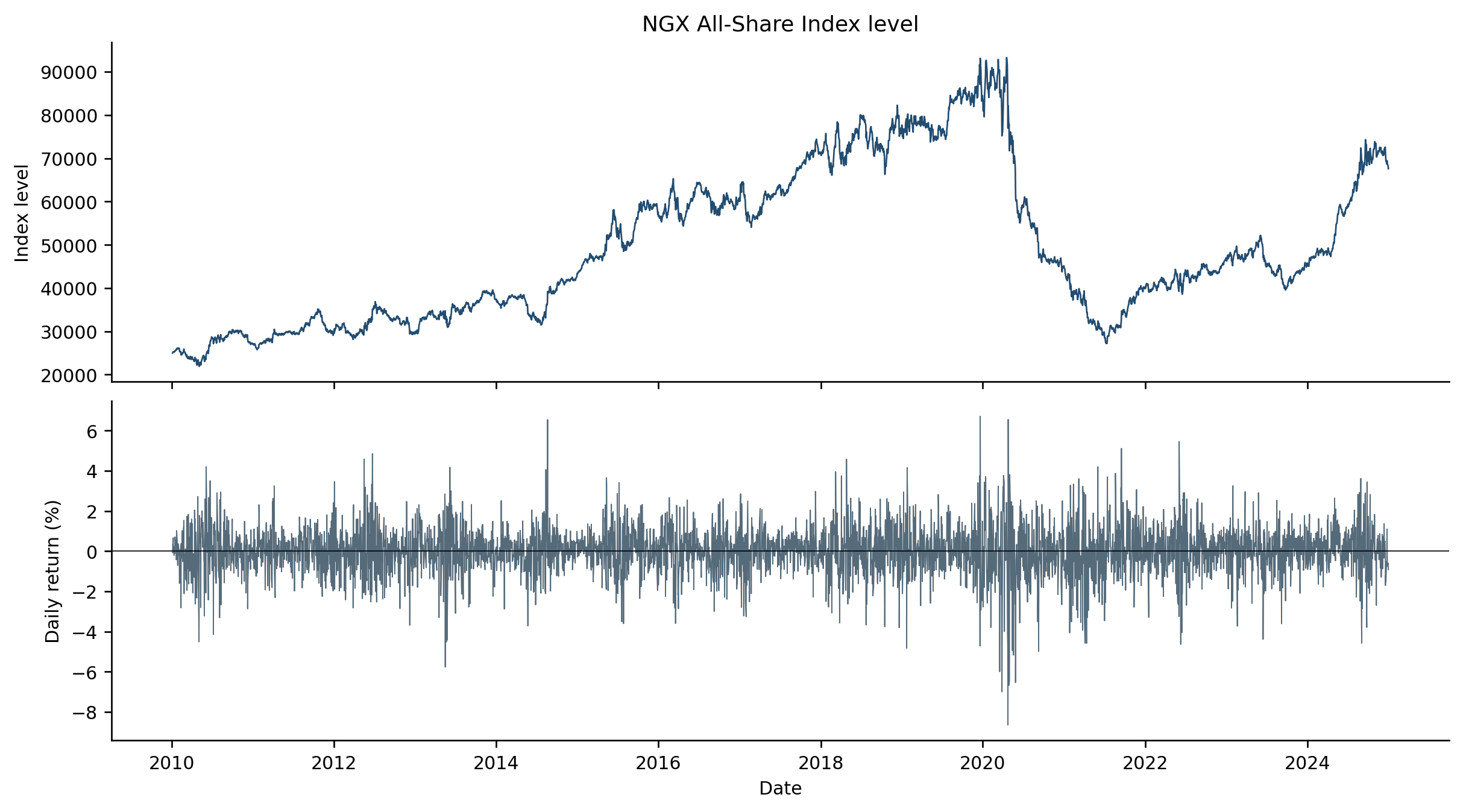
The series contains 3,912 observations. The daily return mean was 0.025% and the standard deviation was 1.254%. Skewness was −0.322, Pearson kurtosis was 6.207, and returns ranged from −8.657% to 6.712%. The Jarque-Bera statistic was 1,738.52 (p < .001). Table 2 reports the descriptive statistics, and Figure 1 shows the index-level and return series.
| Statistic | N | Mean (%) | SD (%) | Skewness | Kurtosis | Minimum (%) / Maximum (%) |
|---|---|---|---|---|---|---|
| Daily return | 3912 | 0.025 | 1.254 | −0.322 | 6.207 | −8.657 / 6.712 |
Note: Kurtosis is reported as Pearson kurtosis, for which the normal benchmark is 3. The Jarque-Bera statistic is 1,738.52 (p < .001). Returns are expressed in percentage units.
4.2Stationarity and ARCH-effect test results
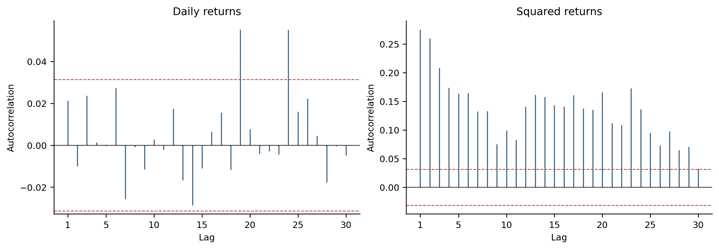
The augmented Dickey-Fuller statistic for returns was −61.205 with zero selected lagged differences (p < .001). The KPSS statistic was 0.173, below the 10% level-stationarity critical value of 0.347. The ten-lag ARCH-LM statistic was 531.875 (p < .001). Figure 2 presents the return and squared-return autocorrelograms.
| Test | Specification | Statistic | Reference value | p-value |
|---|---|---|---|---|
| ADF | Intercept; AIC lag = 0 | −61.205 | 1% critical ≈ −3.43 | < .001 |
| KPSS | Level stationarity; bandwidth 15 | 0.173 | 10% critical = 0.347 | > .10 |
| ARCH-LM | Mean residuals; 10 lags | 531.875 | χ2(10) | < .001 |
Note: ADF and KPSS statistics are computed on daily returns. The ARCH-LM test evaluates the null of no conditional heteroskedasticity.
4.3Model parameter estimates
The GARCH estimates were α = 0.1152 and β = 0.8735, with α + β = 0.9887. The EGARCH estimate for β was 0.9750, and the signed innovation coefficient was γ = −0.0262 (SE = 0.0117). The state-space estimates were φ = 0.9813 and q = 0.0270. Table 4 reports estimates and standard errors for the fitted parameters.
| Model | Parameter | Estimate | Standard error |
|---|---|---|---|
| GARCH(1,1) | Mean, μ | 0.0371 | 0.0178 |
| GARCH(1,1) | ω | 0.0265 | 0.0063 |
| GARCH(1,1) | α | 0.1152 | 0.0123 |
| GARCH(1,1) | β | 0.8735 | 0.0127 |
| EGARCH(1,1) | Mean, μ | 0.0283 | 0.0088 |
| EGARCH(1,1) | ω | 0.0125 | 0.0033 |
| EGARCH(1,1) | α | 0.2217 | 0.0207 |
| EGARCH(1,1) | β | 0.9750 | 0.0051 |
| EGARCH(1,1) | γ | −0.0262 | 0.0117 |
| State-space SV | Long-run log variance, μh | 0.0827 | 0.1603 |
| State-space SV | Persistence, φ | 0.9813 | 0.0054 |
| State-space SV | State variance, q | 0.0270 | 0.0072 |
Note: Estimates are based on 3,129 training observations. GARCH persistence α + β = 0.9887. For EGARCH, γ < 0 indicates a larger estimated log-variance response to negative innovations. The state-space observation-error variance is fixed by the log-chi-square approximation.
4.4Residual diagnostics and in-sample fit
The GARCH standardized-return residuals had Ljung-Box Q(10) = 6.36 (p = .784), and squared residuals had Q(10) = 9.34 (p = .500). The EGARCH values were 6.70 (p = .754) and 10.59 (p = .390), respectively. ARCH-LM statistics were 9.09 (p = .524) for GARCH and 10.26 (p = .418) for EGARCH. State-space measurement-innovation Q(10) and squared-innovation Q(10) statistics were 4.92 (p = .896) and 4.50 (p = .922). Table 5 reports fit statistics.
| Model | Q(10), p | Q2(10), p | ARCH-LM(10), p | Log likelihood | AIC | BIC |
|---|---|---|---|---|---|---|
| GARCH(1,1) | 6.36, .784 | 9.34, .500 | 9.09, .524 | −4855.67 | 9719.34 | 9743.53 |
| EGARCH(1,1) | 6.70, .754 | 10.59, .390 | 10.26, .418 | −4852.59 | 9715.19 | 9745.43 |
| State-space SV | 4.92, .896 | 4.50, .922 | 4.62, .915 | −7088.08 | 14182.16 | 14200.31 |
Note: Q and Q2 tests use standardized return residuals for GARCH and EGARCH, and standardized log-squared-return measurement innovations for state-space SV. State-space likelihood criteria are based on a transformed observation and are not directly comparable with return-density criteria.
4.5Estimated volatility paths
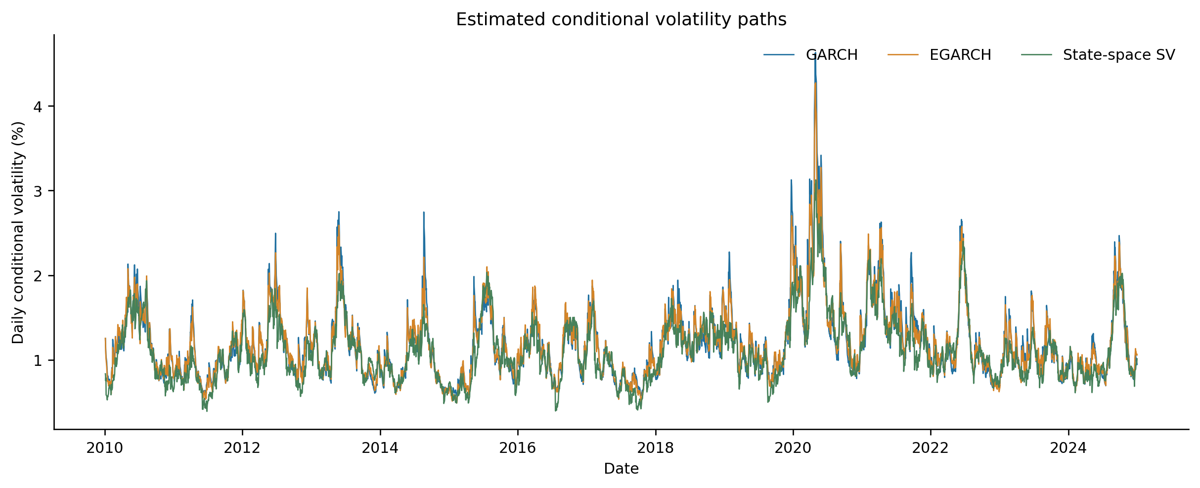
Figure 3 plots the three estimated daily conditional-volatility paths on the same dates and scale. The highest paths occur around the two elevated-volatility episodes in the series. GARCH, EGARCH, and state-space SV each produce time-varying estimates, with differences in the width and timing of several peaks.
4.6Out-of-sample forecast accuracy
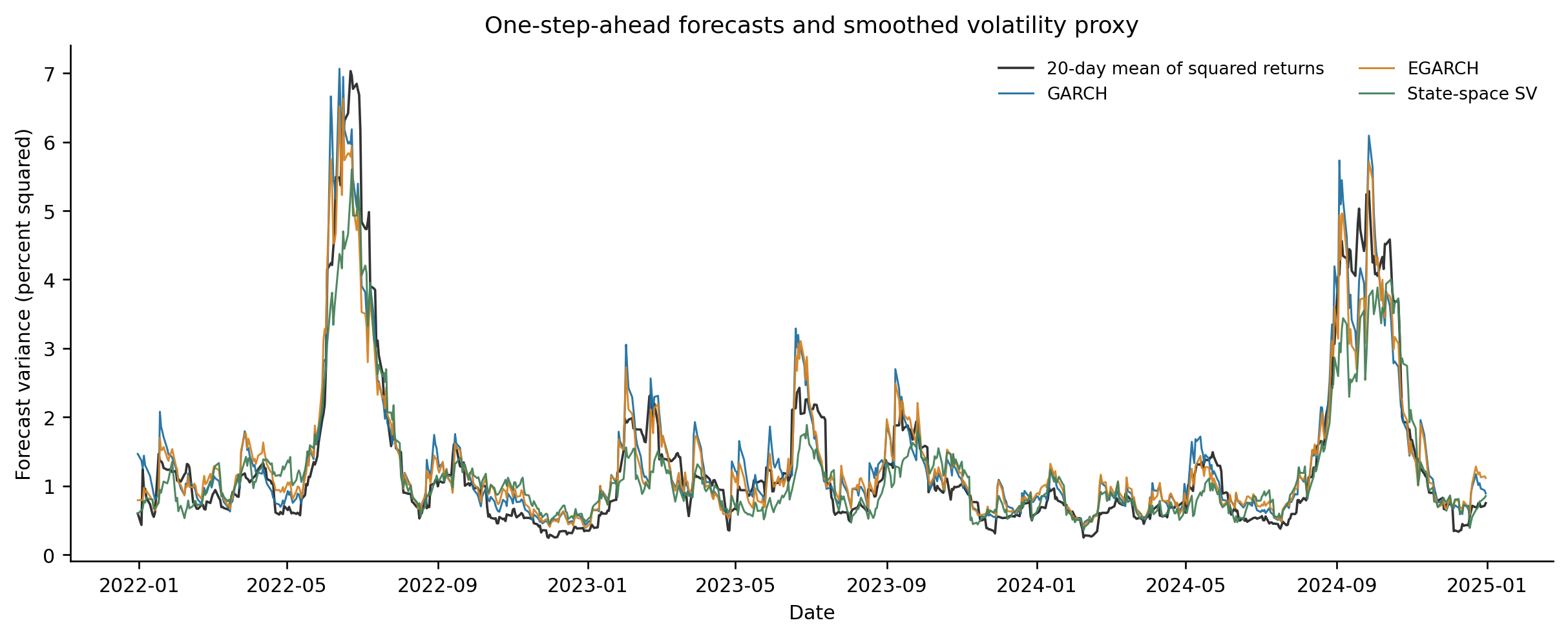
GARCH had the lowest QLIKE score at 1.1071, followed by EGARCH at 1.1076 and state-space SV at 1.1428. EGARCH had the lowest RMSE at 2.4182, while state-space SV had the lowest MAE at 1.2813. The state-space QLIKE loss exceeded the GARCH and EGARCH losses in pairwise tests (DM = 2.404, p = .016; DM = 2.398, p = .017). The GARCH-EGARCH QLIKE difference was not statistically distinguishable (DM = −0.106, p = .916). Table 6 and Figure 4 present the forecast results.
| Model | QLIKE | RMSE | MAE |
|---|---|---|---|
| GARCH(1,1) | 1.1071 | 2.4277 | 1.3445 |
| EGARCH(1,1) | 1.1076 | 2.4182 | 1.3379 |
| State-space SV | 1.1428 | 2.4524 | 1.2813 |
Note: Forecasts are one step ahead for 783 holdout dates. QLIKE is the primary score. Pairwise QLIKE Diebold-Mariano tests with a five-lag Newey-West variance: state-space SV versus GARCH, DM = 2.404, p = .016; state-space SV versus EGARCH, DM = 2.398, p = .017; GARCH versus EGARCH, DM = −0.106, p = .916.
4.7Robustness results
GARCH QLIKE was 1.1071 under Gaussian innovations and 1.1074 under Student-t innovations; EGARCH QLIKE was 1.1076 and 1.1080, respectively. State-space SV QLIKE changed from 1.1428 to 1.1364, its RMSE from 2.4524 to 2.4588, and its MAE from 1.2813 to 1.3413. Table 7 reports the baseline and Student-t scores.
| Model specification | QLIKE | RMSE | MAE |
|---|---|---|---|
| GARCH, Gaussian | 1.1071 | 2.4277 | 1.3445 |
| GARCH, Student-t | 1.1074 | 2.4292 | 1.3488 |
| EGARCH, Gaussian | 1.1076 | 2.4182 | 1.3379 |
| EGARCH, Student-t | 1.1080 | 2.4197 | 1.3420 |
| State-space SV, Gaussian | 1.1428 | 2.4524 | 1.2813 |
| State-space SV, Student-t moments | 1.1364 | 2.4588 | 1.3413 |
Note: Training-sample Student-t degrees of freedom were 8.82 for GARCH, 8.93 for EGARCH, and 10.72 for state-space SV. The state-space specification uses Student-t log-square moments with a Gaussian measurement-error approximation. Scores use the same holdout dates and squared-return proxy as Table 6.
5Discussion
5.1Interpretation of volatility clustering and persistence
GARCH persistence was 0.9887, EGARCH β was 0.9750, and state-space φ was 0.9813. Each indicates slow variance mean reversion, consistent with clustered volatility in Nigerian index and stock studies, though the parameters are not directly interchangeable across models (Emenogu et al., 2020; Adi et al., 2023). Persistence estimates also vary with assets and regimes (Adegboyo & Sarwar, 2025; Haruna Umar & Adeoye, 2020).
5.2Interpretation of asymmetric effects
The negative EGARCH coefficient was statistically different from zero (γ = −0.0262, SE = 0.0117, p = .024), indicating a larger log-variance response to negative innovations of equal magnitude. This direction agrees with Nigerian index evidence, while transition EGARCH and firm-level results show that asymmetry remains asset-specific (Adegboyo & Sarwar, 2025; Tasi’u et al., 2024; Olugbode & Shittu, 2024; Mohammed et al., 2022; Ugomma, 2024).
5.3Comparison of model fit and forecast performance
EGARCH has the lower AIC, while GARCH has the lower BIC; residual diagnostics show no remaining ARCH effect at conventional levels. State-space fit criteria use a transformed observation and are not ranked against return-density criteria.
Forecast rankings depend on loss: GARCH has the lowest QLIKE, EGARCH the lowest RMSE, and SV the lowest MAE. GARCH and EGARCH are indistinguishable under QLIKE, while SV loss is higher than both. This differs from Shuaibu’s (2026) monthly Nigerian result and accords with evidence that rankings vary by horizon and regime (Sahiner, 2022; Wawire et al., 2026).
Different rankings across QLIKE, RMSE, and MAE also appear in cross-market comparisons. Heteroskedasticity-aware tests are relevant to the loss differences; here they separate the close GARCH-family scores from the larger SV QLIKE gap (Xu & Lien, 2022; Fałdziński et al., 2021; Harvey et al., 2024).
QLIKE was the prespecified primary loss, and the pairwise tests support higher loss for state-space SV than for each GARCH-family model, but not a difference between GARCH and EGARCH. RMSE and MAE give a different descriptive ordering: EGARCH had the lowest RMSE and state-space SV the lowest MAE. Because no pairwise tests were reported for RMSE or MAE, those rankings do not establish statistically significant superiority on those losses. This keeps the decision claim tied to the forecast measure with inferential support.
5.4Comparison with Nigerian and related-market studies
Nigerian studies of market-capitalization returns, holidays, and sub-indices report different preferred variants and error laws, reinforcing that firm results do not automatically generalize to an aggregate index (Ahmed et al., 2025; Tasi’u et al., 2024; Adi et al., 2023; Toby & Austen, 2021).
The state-space result depends on its observation equation and filter. Kalman quasi-likelihood and particle filters target different volatility structures, so results from realized volatility or other assets do not predict NGX performance (Asai, 2023; Bégin & Zafari, 2025; Azman et al., 2022; Damian & Frey, 2024).
Shuaibu’s monthly result and this daily result address different forecast designs. Frequency, return aggregation, innovation distribution, the log-square observation equation, and the holdout period can alter volatility persistence and forecast losses. The difference therefore does not establish that either model class is universally superior; it points to design sensitivity that warrants evaluation with observed daily NGX returns and alternative filters (Shuaibu, 2026; Rezende, 2022; Asai, 2023).
5.5Implications for stock-market analysis and risk management
For this design, GARCH leads under QLIKE, EGARCH has the lowest RMSE and an asymmetric response, and SV has the lowest MAE. Model choice should reflect the risk decision and its loss function, not flexibility alone. A QLIKE-focused risk application would retain GARCH as the benchmark and test EGARCH where asymmetric responses matter; the state-space model remains relevant for latent-state estimation but is not preferred here for one-step QLIKE accuracy. Trading volume and market segments may add information, but extensions should preserve an out-of-sample test (Cornelius et al., 2024; Gbadebo, 2023; Pallotta & Ciciretti, 2024; Özgül, 2025).
5.6Contribution, limitations, and future research
The common daily comparison includes fit, diagnostics, forecast scores, and a Student-t check. Its limitations are the constructed index-scale series, squared-return proxy, and Gaussian approximation to the log-square observation (Mao et al., 2020; Rezende, 2022). Because the index-scale sequence is constructed, the results describe this model design and do not establish forecast performance on observed NGX closes. Weekdays are used without a separate exchange-holiday calendar, and daily squared returns are noisy measures of latent variance. Validation with observed exchange data, a trading-day calendar, and intraday realized variance is needed before applying the rankings to market or risk decisions. Further work can compare particle or Bayesian filtering and multiple forecast horizons under the same holdout and loss design.
6Conclusion
All three models estimated persistent volatility, and EGARCH also indicated a negative asymmetric response. Forecast rankings depended on the loss function: GARCH had the lowest QLIKE, EGARCH the lowest RMSE, and state-space SV the lowest MAE. Under QLIKE, state-space forecasts lagged both benchmarks, while GARCH and EGARCH were statistically indistinguishable. The results support evaluating state-space flexibility against common out-of-sample benchmarks and a loss function aligned with the intended risk decision.
References
- [1]Abbara O, Zevallos M (2023a). Estimation and forecasting of long memory stochastic volatility models. Studies in Nonlinear Dynamics & Econometrics, 27(1), 1–24. https://doi.org/10.1515/snde-2020-0106
- [2]Abbara O, Zevallos M (2023b). Maximum likelihood inference for asymmetric stochastic volatility models. Econometrics, 11(1), Article 1. https://doi.org/10.3390/econometrics11010001
- [3]Adegboyo OS, Sarwar K (2025). Modelling and forecasting of Nigeria stock market volatility. Future Business Journal, 11(1), Article 124. https://doi.org/10.1186/s43093-025-00536-4
- [4]Adi AA, Adimani WE, Adda SP (2023). Modelling volatility of sub-indices returns of Nigerian Stock Exchange using GARCH model. Empirical Economic Review, 6(2), 116–134. https://doi.org/10.29145/eer.62.06
- [5]Ahmed I, Adenomon MO, Abdullahi HM, Nweze NO (2025). Modelling the volatility of stock exchange market capitalization returns in Nigeria using GARCH models. Science World Journal, 20(3), 1218–1224. https://doi.org/10.4314/swj.v20i3.42
- [6]Asai M (2023). Estimation of realized asymmetric stochastic volatility models using Kalman filter. Econometrics, 11(3), Article 18. https://doi.org/10.3390/econometrics11030018
- [7]Azman S, Pathmanathan D, Thavaneswaran A (2022). Forecasting the volatility of cryptocurrencies in the presence of COVID-19 with the state-space model and Kalman filter. Mathematics, 10(17), Article 3190. https://doi.org/10.3390/math10173190
- [8]Bégin JF, Zafari G (2025). Estimation of multifactor stochastic volatility jump-diffusion models: A marginalized filter approach. Econometrics and Statistics. Advance online publication. https://doi.org/10.1016/j.ecosta.2025.03.002
- [9]Chau TTT, Ailliot P, Monbet V, Tandeo P (2023). Comparison of simulation-based algorithms for parameter estimation and state reconstruction in nonlinear state-space models. Discrete and Continuous Dynamical Systems - S, 16(2), 240–264. https://doi.org/10.3934/dcdss.2022054
- [10]Chen CWS, Lin EMH, Huang TFJ (2022). Bayesian quantile forecasting via the realized hysteretic GARCH model. Journal of Forecasting, 41(7), 1317–1337. https://doi.org/10.1002/for.2876
- [11]Conrad C, Kleen O (2020). Two are better than one: Volatility forecasting using multiplicative component GARCH-MIDAS models. Journal of Applied Econometrics, 35(1), 19–45. https://doi.org/10.1002/jae.2742
- [12]Cornelius A, OlaOluwa YS, Johnson OF, Damola AM, Omoyeni OT (2024). Trading volume, intraday and overnight volatility of stock returns in the Nigerian Stock Exchange. Asian Journal of Probability and Statistics, 26(9), 110–122. https://doi.org/10.9734/ajpas/2024/v26i9649
- [13]Damian C, Frey R (2024). Detecting rough volatility: A filtering approach. Quantitative Finance, 24(10), 1493–1508. https://doi.org/10.1080/14697688.2024.2399284
- [14]Emenogu NG, Adenomon MO, Nweze NO (2020). On the volatility of daily stock returns of Total Nigeria Plc: Evidence from GARCH models, value-at-risk and backtesting. Financial Innovation, 6(1), Article 18. https://doi.org/10.1186/s40854-020-00178-1
- [15]Fałdziński M, Fiszeder P, Orzeszko W (2021). Forecasting volatility of energy commodities: Comparison of GARCH models with support vector regression. Energies, 14(1), Article 6. https://doi.org/10.3390/en14010006
- [16]Gbadebo AD (2023). Exchange rate volatility and Nigerian stock market development. International Journal of Professional Business Review, 8(9), Article e03078. https://doi.org/10.26668/businessreview/2023.v8i9.3078
- [17]Gong C, Stoffer DS (2021). A note on efficient fitting of stochastic volatility models. Journal of Time Series Analysis, 42(2), 186–200. https://doi.org/10.1111/jtsa.12561
- [18]Gregoir S, Meddahi N (2025). Towards identification of shocks in linear state-space models: Application to stochastic volatility model. Journal of Time Series Analysis, 46(6), 1205–1223. https://doi.org/10.1111/jtsa.70012
- [19]Guzman IE, Ccori PC (2020). A new method for sequential learning of states and parameters for state-space models: The particle swarm learning optimization. Journal of Statistical Computation and Simulation, 90(11), 2057–2079. https://doi.org/10.1080/00949655.2020.1762600
- [20]Haruna Umar Y, Adeoye M (2020). A Markov regime switching approach of estimating volatility using Nigerian stock market. American Journal of Theoretical and Applied Statistics, 9(4), Article 80. https://doi.org/10.11648/j.ajtas.20200904.11
- [21]Harvey DI, Leybourne SJ, Zu Y (2024). Tests for equal forecast accuracy under heteroskedasticity. Journal of Applied Econometrics, 39(5), 850–869. https://doi.org/10.1002/jae.3050
- [22]Kalovwe SK, Mwaniki JI, Simwa RO (2021). On stock returns volatility and trading volume of the Nairobi Securities Exchange Index. RMS: Research in Mathematics & Statistics, 8(1), Article 1889765. https://doi.org/10.1080/27658449.2021.1889765
- [23]Kawakatsu H (2023). Simple factor realized stochastic volatility models. Journal of Time Series Econometrics, 15(1), 79–110. https://doi.org/10.1515/jtse-2021-0049
- [24]Lux T (2022). Inference for nonlinear state-space models: A comparison of different methods applied to Markov-switching multifractal models. Econometrics and Statistics, 21, 69–95. https://doi.org/10.1016/j.ecosta.2020.03.001
- [25]Mahatma Y, Hadi I (2021). Stochastic volatility estimation of stock prices using the Ensemble Kalman Filter. InPrime: Indonesian Journal of Pure and Applied Mathematics, 3(2), 136–143. https://doi.org/10.15408/inprime.v3i2.20256
- [26]Mao X, Czellar V, Ruiz E, Veiga H (2020). Asymmetric stochastic volatility models: Properties and particle filter-based simulated maximum likelihood estimation. Econometrics and Statistics, 13, 84–105. https://doi.org/10.1016/j.ecosta.2019.08.002
- [27]Mohammed T, Umar YH, Adams SO (2022). Modeling the volatility for some selected beverages stock returns in Nigeria (2012–2021): A GARCH model approach. Matrix Science Mathematic, 6(2), 41–51. https://doi.org/10.26480/msmk.02.2022.41.51
- [28]Nemushungwa AI (2024). Assessing the forecasting performance of GARCH models in the presence of instabilities. Universal Journal of Accounting and Finance, 12(1), 13–23. https://doi.org/10.13189/ujaf.2024.120102
- [29]Olugbode MA, Shittu OI (2024). Transition E-GARCH model for modeling and forecasting volatility of equity stock returns in Nigeria Stock Exchange. International Journal of Research and Innovation in Social Science, 7(12), 2120–2134. https://doi.org/10.47772/ijriss.2023.7012162
- [30]Özgül A (2025). GAS or GARCH: A comparison of density and VaR forecasts in Turkish FX and stock markets. Istanbul Business Research, 54(1), 58–86. https://doi.org/10.26650/ibr.2025.54.1577152
- [31]Pallotta A, Ciciretti V (2024). Should you use GARCH models for forecasting volatility? A comparison to GRU neural networks. Studies in Nonlinear Dynamics & Econometrics, 28(5), 725–738. https://doi.org/10.1515/snde-2022-0025
- [32]Pérez-Vieites S, Míguez J (2021). Nested Gaussian filters for recursive Bayesian inference and nonlinear tracking in state-space models. Signal Processing, 189, Article 108295. https://doi.org/10.1016/j.sigpro.2021.108295
- [33]Rezende T (2022). A new filtering inference procedure for a GED state-space volatility model. Journal of Statistical Planning and Inference, 221, 55–68. https://doi.org/10.1016/j.jspi.2022.02.009
- [34]Sahiner M (2022). Forecasting volatility in Asian financial markets: Evidence from recursive and rolling window methods. SN Business & Economics, 2(10), Article 157. https://doi.org/10.1007/s43546-022-00329-9
- [35]Shuaibu H (2026). Forecasting Nigerian equity volatility: A comparative assessment of GARCH, EGARCH, and stochastic volatility models. Gusau Journal of Business Administration, 5(1), 355–367. https://doi.org/10.57233/gujoba.v5i1.30
- [36]Szczepocki P (2023). Estimation of Yu and Meyer bivariate stochastic volatility model by iterated filtering. Przegląd Statystyczny, 2022(4), 1–19. https://doi.org/10.59139/ps.2022.04.1
- [37]Tasi’u M, Umar AA, Abdulaziz U, David RO (2024). Forecasting performance of some GARCH models on holiday-induced volatility in Nigeria Stock Exchange price returns under different error distributions. FUDMA Journal of Sciences, 8(6), 349–353. https://doi.org/10.33003/fjs-2024-0806-3118
- [38]Toby A, Austen G (2021). Volatility modelling of stock returns in the petroleum marketing sector of the Nigerian Stock Exchange. American Journal of Finance, 6(1), 71–97. https://doi.org/10.47672/ajf.777
- [39]Ugomma CA (2024). Evaluation of stock price volatility of MTN and Airtel in Nigeria stock markets. European Journal of Theoretical and Applied Sciences, 2(2), 692–701. https://doi.org/10.59324/ejtas.2024.2(2).60
- [40]Uguru NE, Enwere GM, Amos W (2024). The nexus between exchange rate volatility and Nigerian stock prices: An EGARCH approach. African Journal of Economics and Sustainable Development, 7(1), 56–72. https://doi.org/10.52589/ajesd-atak411m
- [41]Wawire AK, Simiyu CN, Laiboni M, Ochenge R (2026). Horizon- and regime-dependent performance of GARCH-type models: Evidence from volatility forecasting in a frontier market. International Journal of Financial Studies, 14(6), Article 148. https://doi.org/10.3390/ijfs14060148
- [42]Xu Y, Lien D (2022). Forecasting volatilities of oil and gas assets: A comparison of GAS, GARCH, and EGARCH models. Journal of Forecasting, 41(2), 259–278. https://doi.org/10.1002/for.2812