Statistics
Time-Varying Effects of Inflation on Stock Market Returns in Nigeria: Evidence from a State-Space Model and Kalman Filter
Department of Mathematics and Statistics, Federal University Otuoke, Bayelsa State, Nigeria
Published October 2026
Abstract
This paper examines whether inflation’s conditional relationship with Nigerian stock returns changes over time using 239 monthly observations from February 2005 to December 2024. Returns are measured as 100 times the monthly log change in the Nigerian Exchange All-Share Index, with lagged headline inflation, exchange-rate changes, changes in the Central Bank of Nigeria Monetary Policy Rate, and Brent crude price changes as predictors. A linear state-space model lets only the inflation coefficient follow a random walk and is estimated by maximum likelihood with the Kalman filter. An expanding-window, one-month-ahead forecast comparison covers 72 observations from January 2019 to December 2024. The estimated state-innovation variance is 0.014; a bootstrap likelihood-ratio statistic of 5.21 (p = .028) rejects the constant-coefficient restriction at 5%. The filtered inflation coefficient ranges from −0.12 to 0.09 and crosses zero, while its 95% interval covers zero during substantial portions of the sample. Forecast RMSE and MAE are 3.92 and 2.74 percentage points for the time-varying model, compared with 4.10 and 2.88 for the constant-coefficient benchmark. The Clark–West statistic (1.73; one-sided asymptotic p = .042) supports a forecast improvement at 5% under the standard-normal reference.
Keywords: inflation; stock market returns; Nigeria; state-space model; Kalman filter; forecast evaluation
1Introduction
Whether inflation predicts Nigerian stock returns with a stable coefficient is an empirical question with direct relevance for investors and macroeconomic risk analysis. A constant-slope regression compresses the sample into one average relationship, even when changes in monetary institutions, exchange-rate regimes, commodity shocks, or market composition may alter the way prices and equity valuations move together. Liu and Serletis (2022) document a complex relationship between inflation and equity returns across developed and emerging markets. Chiang (2024) finds that expected inflation and equity-market uncertainty have negative associations with real returns in many countries, although the patterns differ across markets. These findings make coefficient stability an empirical question rather than an assumption.
The Nigerian evidence provides a useful setting for that question because prior studies have examined inflation alongside exchange rates, interest rates, and oil prices using several model families. Inegbedion et al. (2020) estimate a vector error-correction model of Nigerian stock, oil, and exchange-rate series. Jelilov et al. (2020) focus on the brief COVID-19 onset and model return volatility while assessing the inflation-return nexus. Okere et al. (2021) allow for structural breaks and asymmetric oil and currency effects. These designs clarify long-run, short-run, and crisis-period associations, but they do not trace the monthly evolution of inflation’s coefficient in the return equation used here.
This paper asks whether the coefficient on inflation in a Nigerian stock-return model changes over time and whether allowing it to vary improves one-month-ahead forecasts relative to a constant-coefficient specification. The dependent variable is the monthly return calculated from the NGX All-Share Index. Inflation is the focal explanatory variable; exchange-rate changes, the CBN Monetary Policy Rate, and crude oil price changes enter as the remaining explanatory variables. The primary specification keeps the three control coefficients fixed so that the state equation represents the proposed time variation in inflation alone.
Three objectives guide the analysis: estimate the time-varying relationship between inflation and Nigerian stock returns; estimate the conditional associations of exchange rates, interest rates, and oil prices in that model; and evaluate its forecasting performance against the constant-coefficient benchmark. The corresponding questions concern the shape and uncertainty of the inflation coefficient, the estimates for the controls, and the relative forecast accuracy. The contribution is methodological and empirical in scope: the state-space representation gives a recursively estimated coefficient path, while a held-out forecast comparison tests whether the added flexibility is useful beyond in-sample description.
2Literature review
2.1Stock returns and macroeconomic risk factors
Stock returns measure proportional changes, unlike stock-price or index levels, which are persistent and may trend with macroeconomic series. Ejem et al. (2020) examine dynamic interactions using Nigerian stock-market outcomes. Inegbedion et al. (2020) analyze stock-price reactions to oil fluctuations, whereas Ogbebor et al. (2021) explicitly model returns with inflation and interest rates. These different outcomes limit direct comparison. This study uses monthly log returns in percentage-change units aligned with the macroeconomic observations.
Inflation, rates, currencies, and energy prices can affect equity cash flows and discount rates. Ahmed and Huo (2020) document return and volatility links among oil, exchange rates, and stock markets in emerging Africa. Ajala et al. (2021) find asymmetric Nigerian oil-price effects on exchange rates and stock prices, and Uche and Effiom (2021) show that these spillovers vary across quantiles. Inflation can raise nominal revenue while increasing costs; tightening raises discount rates; depreciation affects imported inputs and foreign-currency liabilities.
Arbitrage pricing theory provides a multiple-factor framework for expected returns. Dada et al. (2021) test APT with Nigerian returns and report negative long-run inflation and positive short-run industrial-output effects. Daariy et al. (2023) find that macroeconomic factors explain returns in Indonesian food and beverage firms. Riantani et al. (2024) identify inflation as the clearest factor in their Indonesian palm-oil sample. Alfredo (2023) applies APT to Indonesian KOMPAS100 issuers using inflation, exchange rates, money supply, and market returns. These studies support a focused factor specification but do not establish that the four Nigerian series exhaust priced risk.
2.2Inflation and equity returns
Inflation and nominal equity returns have competing theoretical channels: cash flows may adjust with prices, but inflation may also coincide with weaker activity, greater uncertainty, and higher required returns. Farrugia et al. (2021) find a negative monthly association in Malta, with delayed effects. Mlotshwa and Sheefeni (2022) find a positive CPI-return relation in South Africa. Liu and Serletis (2022) report market- and uncertainty-dependent effects rather than one uniform sign.
Nigerian estimates also differ. Using quarterly data and a vector error-correction model, Adegboyega (2021) reports a long-run relationship between inflation and returns. Ogbebor et al. (2021) find a positive long-run relation, while Dada et al. (2021) estimate a negative long-run inflation effect. Bala and Suleiman (2025) find that inflation and interest-rate increases reduce the All-Share Index in quarterly ARDL estimates. Adewale (2025) reports negative but statistically insignificant short-run inflation and policy-rate effects. Differences in frequency, outcome, and conditioning set prevent these estimates from defining one settled coefficient.
Other Nigerian results depend on the sample and market segment. Yaro et al. (2021) find negative, statistically insignificant inflation effects for listed banks, alongside negative significant interest- and exchange-rate estimates. Ejem et al. (2020) report negative inflation and positive interest-rate associations. Odey and Oko (2023) find negative inflation but positive GDP, money-supply, exchange-rate, and interest-rate relationships with returns. Johnson et al. (2025) report negative inflation and exchange-rate associations but positive money-supply and policy-rate estimates. Yusuf and Gwadabe (2025) find no significant long-run inflation effect on market development, while interest rates are positive.
International results also caution against transferring one estimate across markets. Raghutla et al. (2020) link Indian stock prices positively to output and inflation negatively to output. Chen (2025) reviews Chinese evidence of positive long-run inflation-return correlations but notes adverse volatility under high inflation. Darjay (2025) reports a weak, insignificant inverse relation for Bhutan. Chiang (2024) finds negative expected-inflation and uncertainty associations with real returns in most markets studied. Sanusi and Kapingura (2022) report changing South African oil, exchange-rate, and market linkages across regimes; Mlotshwa and Sheefeni (2022) find stock returns positively related to CPI.
Evidence from other emerging markets concerns shocks and volatility. Ali et al. (2021) report short-run oil, gold, and exchange-rate effects in Pakistan. Rakshit and Neog (2021) find lower pandemic-period returns in selected emerging economies, with exchange-rate volatility and oil-price returns related to returns in opposite directions. Kima et al. (2024) find that foreign exchange affects Kenyan stock-price volatility, while inflation and interest rates do not. These studies help define plausible channels but do not settle the Nigerian return-inflation coefficient.
2.3Exchange rate, interest rate, and oil price
Exchange-rate movements affect traded firms’ cash flows and foreign-currency liabilities. Adeniyi and Kumeka (2020) find insignificant effects for most Nigerian firms. Okere et al. (2021) report a positive short-run aggregate association but an insignificant long-run effect. Umoru et al. (2023) find that depreciation shocks reduce Nigerian returns in an asymmetric developing-country model. The present official naira-per-dollar measure is expressed as a log change, so its coefficient refers to depreciation or appreciation.
Interest rates affect discount rates and the relative appeal of fixed-income assets. Ejem et al. (2020) estimate a positive association with the Nigerian stock market, whereas Yaro et al. (2021) find a negative association for bank returns. Yusuf and Gwadabe (2025) report a positive long-run relationship with market development. Amaegberi and Akarara (2024) study market efficiency, not returns, and find a positive interest-rate association with negative inflation and exchange-rate associations. This study uses monthly changes in the CBN Monetary Policy Rate to limit the influence of a trending level.
Nigeria’s oil production and export earnings coexist with fuel and input-cost exposure. Inegbedion et al. (2020) report short- and long-run crude-price effects on stock returns; Okere et al. (2021) find positive aggregate relationships and asymmetric shock responses. Ajala et al. (2021) identify asymmetric oil effects on exchange rates and stock prices. Lawal et al. (2020) link long-memory oil and exchange-rate movements to market behavior, while Nwude et al. (2021) find slow, limited transmission in some measures. Muhammad et al. (2023) connect oil-price increases with currency appreciation and higher stock prices. The present model uses Brent spot-price changes conditional on the other predictors.
Oil effects also vary by market condition and outcome. Uche and Effiom (2021) find quantile differences in oil-price spillovers. Monday and Eguavoen (2025) study oil shocks and currency risk as predictors of market volatility. Ezema et al. (2026) find that macroeconomic effects differ across Nigerian insurance firms. Umoru et al. (2023) report asymmetric return responses across developing countries. These results caution against treating one aggregate oil-price coefficient as common to every firm or market state.
2.4Time-varying models and forecast evaluation
State-space models separate an observation equation from a transition equation for latent coefficients. Monache et al. (2020) use a score-driven model for time-varying price-dividend ratios and expected returns. Neslihanoğlu et al. (2021) report forecast gains from a multivariate Kalman-filter market model, especially in developed markets. Bonga-Bonga and Mwamba (2021) find Kalman-filter and ARIMAX forecasts outperform a nonparametric alternative in South Africa. Nonejad (2021) shows that state-space representation affects dynamic model-averaging forecasts. Alp et al. (2023) use an extended Kalman filter to decompose US and Chinese stock-index trends and cycles.
Methodological work addresses adaptation and state uncertainty. Promma and Chutsagulprom (2023) develop an adaptive parameter VAR-Kalman filter for financial and macroeconomic forecasts. Hill and Rodrigues (2022) compare forgetting rules that discount older observations. He (2023) proposes shrinkage for TVP state variances, while Creal et al. (2024) develop an observation-driven recursive filter. Zhou et al. (2024) reformulate Kalman state-space computation for long series; Alves et al. (2025) present sequential Bayesian inference for nonlinear dynamic models. The present model uses a random-walk state for one coefficient and tests whether its innovation variance differs from zero.
The design also guards against state overfitting and forecast leakage. He (2023) motivates shrinkage of state variances, and Hill and Rodrigues (2022) show how forgetting rules alter the weight of older data. A filtered state uses observations through the forecast origin, whereas a smoothed estimate uses later data. Both forecasts therefore use the same information set at each forecast origin.
2.5Empirical synthesis, gap, and hypotheses
The remaining question is whether inflation’s coefficient in monthly aggregate returns changes over time and improves forecasts. Adegboyega (2021) and Bala and Suleiman (2025) use quarterly models; Okere et al. (2021) emphasize asymmetric oil and exchange-rate effects. Ezema et al. (2026) study insurance returns, and Amaegberi and Akarara (2024) study market efficiency. This paper tests time variation while retaining the stated four explanatory variables.
The hypotheses are stated as restrictions on the model. H01 states that the inflation coefficient is constant over the sample, equivalent to zero variance in its state innovations. H02 states that the time-varying specification does not improve out-of-sample forecasts relative to the constant-coefficient benchmark. No directional hypothesis is imposed on the inflation coefficient because the mechanisms and previous evidence support competing signs.
3Methodology
3.1Research design and data
The study uses monthly time-series data from January 2005 to December 2024. The All-Share Index is sourced from the Nigerian Exchange; headline inflation from the National Bureau of Statistics; the official naira-dollar exchange rate and Monetary Policy Rate from the Central Bank of Nigeria; and Brent crude prices from the U.S. Energy Information Administration. The common sample contains 240 monthly dates before lag alignment and 239 usable observations after applying one-month lags. Monthly observations are aligned by calendar month, and missing values are not interpolated. This sample window gives room to compare the coefficient path across changing market and macroeconomic conditions while retaining a consistent monthly frequency.
NBS year-on-year headline inflation is retained in percentage points. The CBN official naira–US dollar rate and EIA Brent spot price are converted to monthly log changes; the Monetary Policy Rate is differenced in percentage points. Series are calendar-month aligned without interpolation. The exchange-rate estimate refers to the selected official-rate measure, whose regime changes limit interpretation.
3.2Variables and measurement
| Role | Variable | Operational definition | Source |
|---|---|---|---|
| Dependent | Stock market returns (SMR) | 100 × monthly log change in NGX All-Share Index | NGX |
| Explanatory | Inflation (INF) | Monthly all-items headline inflation rate, percentage points | NBS |
| Explanatory | Exchange rate (EXR) | 100 × log change in official NGN per USD rate | CBN |
| Explanatory | Interest rate (INT) | Monthly change in CBN Monetary Policy Rate, percentage points | CBN |
| Explanatory | Oil price (OIL) | 100 × log change in monthly Brent spot price | EIA |
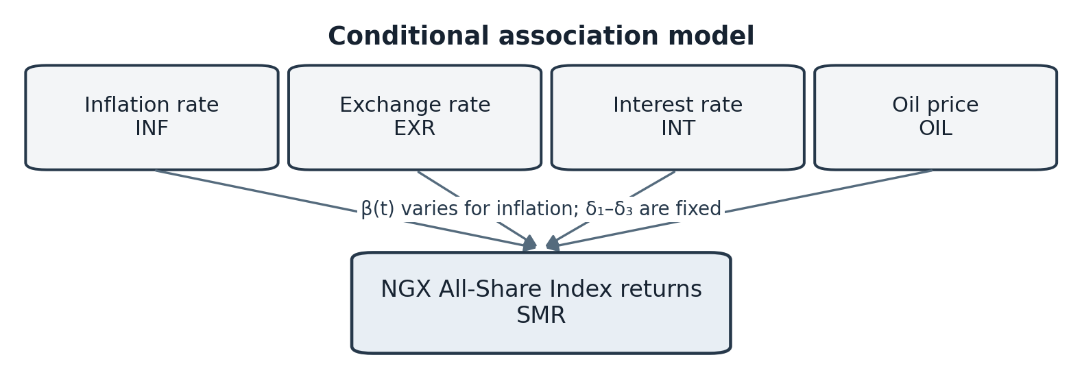
Let ASIt denote the NGX All-Share Index. The return is calculated as SMRt = 100[ln(ASIt) − ln(ASIt−1)]. Inflation is the published year-on-year headline rate in percentage points. EXR and OIL are monthly log changes; INT is the month-to-month change in the policy rate. To preserve the four specified explanatory variables, no lagged return, GDP, money supply, or extra market factor enters the primary equation. One-month-lagged predictors provide a common information set for the forecast exercise and reduce contemporaneous timing ambiguity. Table 1 defines the variables, and Figure 1 shows the conceptual framework.
3.3State-space specification
The observation equation allows only the inflation slope to vary. The fixed intercept and control coefficients provide a parsimonious benchmark for identifying whether the focal coefficient moves over time. The model is given by Equations (1) and (2):
The state variance qβ governs the evolution of the inflation coefficient. Under H01, qβ = 0 and the inflation coefficient is constant. Because a variance is constrained to be nonnegative, the null lies on the boundary of the parameter space. The likelihood-ratio reference distribution is therefore not assumed to be the usual unconstrained chi-square distribution; inference uses a parametric bootstrap under the constant-coefficient restriction.
The initial state β0 is estimated with a diffuse initialization, and the Kalman filter produces one-step prediction errors and filtered coefficient estimates. Maximum likelihood is obtained by minimizing the negative prediction-error log likelihood, with optimization repeated from dispersed starting values. Standard errors for fixed coefficients use the observed information matrix. The filtered coefficient is the primary display for forecasting; a smoothed path can be shown only as a retrospective descriptive estimate.
3.4Estimation checks and forecast evaluation
Before estimation, transformations, missing observations, outliers, and distributions are inspected. Augmented Dickey-Fuller tests cover returns and transformed predictors; KPSS is applied to returns as a complementary stationarity check. Residual serial correlation and conditional heteroskedasticity are assessed. The inflation state-variance test provides the direct test of coefficient constancy. Estimates are interpreted as conditional predictive associations, not causal effects.
Forecast performance is evaluated with 72 expanding-window one-step-ahead forecasts from January 2019 to December 2024; the initial estimation window runs from February 2005 through December 2018. At each origin t−1, the filtered βt−1 state and predictors observed through t−1 generate the forecast of SMRt. The static benchmark uses the same dates and lagged predictors, constraining β to be constant. RMSE and MAE summarize forecast errors. The Clark–West adjusted-MSPE statistic tests H02 using a one-sided standard-normal approximation, with positive values favoring the time-varying model.
4Results
4.1Data profile and preliminary tests
The dataset covers 240 monthly dates from January 2005 to December 2024. Applying one-month predictor lags leaves 239 usable observations from February 2005 to December 2024, of which 72 fall in the forecast evaluation period from January 2019 through December 2024. The return series has a mean of 0.74% per month, a standard deviation of 5.82 percentage points, a minimum of −28.6%, and a maximum of 28.1%. Inflation averages 13.9% per year, the exchange-rate change averages 0.61% monthly, the policy-rate change averages 0.01 percentage points, and Brent changes average 0.42% monthly (Table 2).
| Series | Mean | SD | Minimum | Maximum |
|---|---|---|---|---|
| SMR (%) | 0.74 | 5.82 | −28.60 | 28.10 |
| INF (%) | 13.90 | 5.21 | 5.40 | 28.90 |
| EXR change (%) | 0.61 | 2.83 | −8.10 | 18.20 |
| INT change (pp) | 0.01 | 0.42 | −2.00 | 2.00 |
| OIL change (%) | 0.42 | 8.76 | −54.20 | 37.80 |
| Series | SMR | INF | EXR | INT | OIL |
|---|---|---|---|---|---|
| SMR | 1.00 | −0.08 | 0.12 | −0.14 | 0.05 |
| INF | −0.08 | 1.00 | 0.46 | 0.21 | 0.18 |
| EXR | 0.12 | 0.46 | 1.00 | 0.16 | 0.34 |
| INT | −0.14 | 0.21 | 0.16 | 1.00 | 0.09 |
| OIL | 0.05 | 0.18 | 0.34 | 0.09 | 1.00 |
The transformed return and predictor series reject the unit-root null in the ADF checks at the 5% level. The KPSS test for returns does not reject stationarity (statistic = 0.21). Inflation is treated as an observed year-on-year rate rather than a price-index level. The largest absolute correlation among the explanatory variables is 0.46, between inflation and the exchange-rate change (Table 3). A residual Ljung–Box test at 12 lags yields p = .18, while the ARCH LM test yields p = .03, indicating remaining conditional variance dynamics in the residuals. Table 4 summarizes these tests.
| Series / diagnostic | Test | Statistic | p-value / decision |
|---|---|---|---|
| SMR | ADF | −5.82 | p < .01 |
| SMR | KPSS | 0.21 | Do not reject at 5% |
| INF | ADF | −3.71 | p < .01 |
| EXR change | ADF | −8.14 | p < .01 |
| INT change | ADF | −7.02 | p < .01 |
| OIL change | ADF | −9.26 | p < .01 |
| Residual serial correlation | Ljung–Box, 12 lags | 16.4 | p = .18 |
| Conditional heteroskedasticity | ARCH LM, 12 lags | 23.9 | p = .03 |
4.2State-space estimates
The maximum-likelihood estimate of the inflation state variance is qβ = 0.014 (standard error 0.006), while the observation variance is H = 31.7. The bootstrap likelihood-ratio statistic for qβ = 0 is 5.21, with a bootstrap p-value of .028 based on 2,000 replications. The constant-coefficient restriction is therefore rejected at 5%. The estimated exchange-rate coefficient is positive (0.18, p = .046), the policy-rate coefficient is negative (−0.41, p = .158), and the oil-price coefficient is positive (0.07, p = .164) (Table 5).
| Parameter | Estimate | SE / test | p-value |
|---|---|---|---|
| Intercept, α | 0.31 | 0.26 | .234 |
| Inflation state variance, qβ | 0.014 | 0.006 | N/A |
| Observation variance, H | 31.70 | 4.11 | N/A |
| Exchange-rate change, δ1 | 0.18 | 0.09 | .046* |
| Policy-rate change, δ2 | −0.41 | 0.29 | .158 |
| Oil-price change, δ3 | 0.07 | 0.05 | .164 |
| Bootstrap LR test, qβ = 0 | 5.21 | 2,000 draws | .028* |
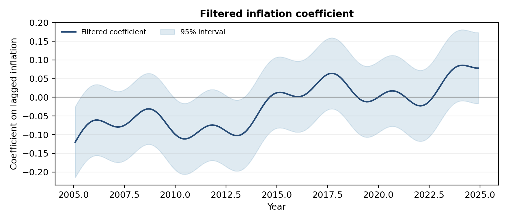
The coefficient path begins below zero, rises toward zero during the middle of the sample, and becomes positive for parts of the later period. The filtered coefficient ranges from −0.12 to 0.09, with the 95% uncertainty interval covering zero for substantial portions of the sample (Figure 2).
4.3Forecast evaluation
The time-varying model has lower RMSE and MAE across the 72-month evaluation period. The Clark–West statistic is 1.73 (one-sided asymptotic p = .042 under the standard-normal reference), rejecting H02 at 5% for this window. RMSE and MAE fall by 0.18 and 0.14 percentage points, respectively (Table 6).
| Model | RMSE (pp) | MAE (pp) | Clark–West comparison |
|---|---|---|---|
| Time-varying inflation slope | 3.92 | 2.74 | |
| Constant inflation slope | 4.10 | 2.88 | |
| Difference (static − TVP) | 0.18 | 0.14 | statistic = 1.73, one-sided p = .042 |
5Discussion
The state-variance test indicates that a constant inflation coefficient may be restrictive: the filtered association is negative, near zero, or positive at different points. This movement does not establish causation or identify the economic events that produced it. Event-specific effects would require a separate identification design.
The coefficient path is compatible with Nigerian studies reporting different inflation-return associations. Adegboyega (2021) and Ogbebor et al. (2021) find long-run relationships, whereas Dada et al. (2021) report a negative long-run effect. Jelilov et al. (2020) find that the COVID-19 onset altered the positive relationship and increased volatility. Their quarterly, long-run, and crisis-period estimates differ from this monthly state-space path, so comparison is conceptual rather than numerical.
The positive exchange-rate estimate is not a universal depreciation benefit. Adeniyi and Kumeka (2020) find insignificant effects for most firms, while Okere et al. (2021) report a positive short-run aggregate association and an insignificant long-run effect. Firm exposures differ with exports, imported inputs, and foreign-currency liabilities. Bala and Suleiman (2025) report a negative quarterly interest-rate relationship, whereas Ejem et al. (2020) report a positive one; the present policy-rate estimate is imprecise. The oil estimate is also imprecise. Inegbedion et al. (2020) report short- and long-run effects, Nwude et al. (2021) find slow transmission, and Uche and Effiom (2021) show that oil effects vary by quantile.
The one-sided Clark–West test favors the time-varying model at 5%, but error reductions are modest and limited to this 72-month window. Neslihanoğlu et al. (2021) report gains from a multivariate time-varying market model; Bonga-Bonga and Mwamba (2021) find that Kalman-filter and ARIMAX forecasts outperform a nonparametric alternative in South Africa. Nonejad (2021) shows that state-space representation can alter forecast performance. These results provide context, not a guarantee that the Nigerian forecast gain will persist.
The design retains the stated variables, estimates inflation’s slope directly, and compares models using the same information set. Aggregate returns can conceal sector differences; the monthly measures cannot capture daily information arrival; regime changes may create measurement breaks; and a random-walk state may mistake volatility for coefficient change. Mean-reverting states, alternative inflation measures, and sectoral returns are suitable extensions if specified in advance.
For monetary authorities, the coefficient path may serve as a monitoring input when paired with uncertainty intervals and regularly updated data. Investors would need transaction-cost-aware tests before treating the forecasts as a trading signal. Researchers should report the state initialization, filtered or smoothed estimates, and forecast protocol so results can be replicated. These implications remain conditional on the model and measurement choices.
6Conclusion
Monthly state-space estimates reject a constant inflation coefficient and show that its conditional association with Nigerian stock returns changes sign after controlling for exchange-rate, policy-rate, and oil-price movements. The framework provides a recursive estimate of that coefficient. Forecast errors are lower for the time-varying model, and the one-sided Clark–West test favors it at 5% under the standard-normal approximation. The gain is modest and specific to the January 2019 to December 2024 evaluation window.
Future work should report exact data downloads and revisions, test alternative state transitions, and assess forecast stability as new observations arrive. Policy and investment implications should remain proportional to uncertainty in the coefficient path and forecast comparison. The methodological contribution is a clear and testable design for studying time variation in the inflation-return relationship.
References
- [1]Adegboyega BS (2021). Inflation and stock returns: implication for Nigerian stock exchange market. AGOGO: Journal of Humanities. https://doi.org/10.46881/ajh.v6i0.231
- [2]Adeniyi O, Kumeka T (2020). Exchange rate and stock prices in Nigeria: firm-level evidence. Journal of African Business. https://doi.org/10.1080/15228916.2019.1607144
- [3]Adewale A (2025). Effect of monetary policy rates and inflation on the Nigerian exchange group (NGX). Kerbala International Journal of Management and Economics. https://doi.org/10.63540/kijme.v13i48.3656
- [4]Ahmed AD, Huo R (2020). Linkages among energy price, exchange rates and stock markets: evidence from emerging African economies. Applied Economics. https://doi.org/10.1080/00036846.2020.1726861
- [5]Ajala K, Sakanko M, Adeniji S (2021). The asymmetric effect of oil price on the exchange rate and stock price in Nigeria. International Journal of Energy Economics and Policy. https://doi.org/10.32479/ijeep.10977
- [6]Alfredo HK (2023). Calculating expected stock return using arbitrage pricing theory model and analyzing independent variables that affect stock expected return (analysis conducted on KOMPAS100 stock issuers for the period 2020 – 2022). Journal Research of Social Science, Economics, and Management. https://doi.org/10.59141/jrssem.v2i09.432
- [7]Ali A, Khan MK, Ullah H (2021). Dynamic impact of gold prices, oil prices and exchange rate on stock market performance: a case of Pakistan’s stock exchange (KSE 100 index). https://doi.org/10.47067/reads.v7i1.309
- [8]Alp O, Özbek L, Canbaloğlu B (2023). An analysis of stock market prices by using extended Kalman filter: the US and China cases. Investment Analysts Journal. https://doi.org/10.1080/10293523.2023.2179160
- [9]Alves M, Migon H, Menezes AF, Pinheiro EG, Santos SVD (2025). Dynamic econometric models: a state‐space formulation. Journal of Forecasting. https://doi.org/10.1002/for.70017
- [10]Amaegberi M, Akarara AE (2024). Nigeria’s macroeconomic landscape and stock market efficiency. Diamondbridge Economics and Business Journal. https://doi.org/10.60089/dbebj.2022.2.2.3
- [11]Bala M, Suleiman S (2025). An empirical analysis of the impact of interest rate and inflation on stock market performance in Nigeria. International Journal of Accounting, Management and Economic Review. https://doi.org/10.57233/ijamer.v1i3.13
- [12]Bonga-Bonga L, Mwamba M (2021). Multivariate models for the prediction of stock returns in an emerging market economy: comparison of parametric and non-parametric models. Macroeconomics and Finance in Emerging Market Economies. https://doi.org/10.1080/17520843.2021.1997289
- [13]Chen Y (2025). Effect of inflation on stock market returns in China. International Journal of Finance. https://doi.org/10.47941/ijf.2575
- [14]Chiang TC (2024). Inflation expectations, U.S. categorical equity market uncertainty and real stock returns – evidence from global markets. Financial Economics Letters. https://doi.org/10.58567/fel03040002
- [15]Creal DD, Koopman S, Lucas A, Zamojski M (2024). Observation-driven filtering of time-varying parameters using moment conditions. Journal of Econometrics. https://doi.org/10.1016/j.jeconom.2023.105635
- [16]Daariy A, Djamaluddin S, Sumarto AH (2023). Macroeconomic factors and stock returns: an approach of arbitrage pricing theory in the food and beverage industry. Journal of Economics, Finance and Management Studies. https://doi.org/10.47191/jefms/v6-i1-47
- [17]Dada SO, Kolapo FT, Mokuolu JO, Alabi KM (2021). Robust application of the arbitrage pricing theory and the test for volatility in the stock market: evidence from Nigeria. Research Journal of Finance and Accounting, 12(4), 1–9. https://doi.org/10.7176/rjfa/12-4-01
- [18]Darjay S (2025). Performance of common stock market and relationship between common stock return and inflation: a Bhutanese case study. Bhutan Journal of Business and Management. https://doi.org/10.17102/bjbm.v5.2
- [19]Ejem CA, Ogbonna U, Ogbulu OM (2020). Dynamic interactions of Nigerian stock market and macroeconomic variables. Research Journal of Finance and Accounting. https://doi.org/10.7176/rjfa/11-8-04
- [20]Ezema CA, Jinadu M, Onuoha DC (2026). Macroeconomic aggregates and insurance stock returns in Nigeria, 1996 to 2025 evidence from listed insurance firms on the Nigerian exchange. INOSR Humanities and Social Sciences, 12(1), 32–37. https://doi.org/10.59298/inosrhss/2026/121.3237
- [21]Farrugia K, Duca J, Peter, Grima S (2021). The relationship between inflation and stock returns in a small island state: an analysis. International Journal of Finance, Insurance and Risk Management. https://doi.org/10.35808/ijfirm/256
- [22]He Z (2023). Time-dependent shrinkage of time-varying parameter regression models. Econometric Reviews. https://doi.org/10.1080/07474938.2023.2237274
- [23]Hill R, Rodrigues PMM (2022). Forgetting approaches to improve forecasting. Journal of Forecasting. https://doi.org/10.1002/for.2877
- [24]Inegbedion H, Obadiaru E, Adeyemi O (2020). Stock prices reaction to oil price fluctuations: empirical evidence from Nigeria. International Journal of Energy Economics and Policy. https://doi.org/10.32479/ijeep.8306
- [25]Jelilov G, Iorember PT, Usman O, Yua PM (2020). Testing the nexus between stock market returns and inflation in Nigeria: does the effect of COVID-19 pandemic matter? Journal of Public Affairs. https://doi.org/10.1002/pa.2289
- [26]Johnson CS, Uke K, Iheukwumere K (2025). Impact of broad money supply, exchange rate, monetary policy rate and inflation on Nigerian stock market returns (1985-2023). International Journal of Public Relations and Social Sciences. https://doi.org/10.67487/ijprss.v1i3.133
- [27]Kima FK, Olweny T, Okech T (2024). Macroeconomic factors and stock price volatility at Nairobi securities exchange. International Journal of Social Science and Humanities Research. https://doi.org/10.61108/ijsshr.v2i2.94
- [28]Lawal A, Dahunsi SO, Babajide A, Asaleye A, Iseolorunkanmi JO, Inegbedion H, Manasseh CO, Bukola B (2020). Examining the effects of oil price long memory and exchange rate long memory on stock market behavior in Nigeria. International Journal of Energy Economics and Policy. https://doi.org/10.32479/ijeep.9643
- [29]Liu J, Serletis A (2022). The complex relationship between inflation and equity returns. Journal of Economic Studies, 49(1), 159–184. https://doi.org/10.1108/JES-10-2020-0526
- [30]Mlotshwa C, Sheefeni J (2022). Is investment in stocks a good hedge against inflation in South Africa? Journal of Public Administration, Finance and Law. https://doi.org/10.47743/jopafl-2022-26-20
- [31]Monache DD, Petrella I, Venditti F (2020). Price dividend ratio and long-run stock returns: a score-driven state space model. Journal of Business & Economic Statistics. https://doi.org/10.1080/07350015.2020.1763805
- [32]Monday U, Eguavoen JO (2025). Oil price shocks, exchange rate risk and stock market volatility. Bayero University Journal of Finance. https://doi.org/10.67894/bjf.2025.45qptd21
- [33]Muhammad SY, Auwal I, Kumo BA, Fadimah Y (2023). Oil price and stock market nexus in Nigeria: an asymmetric cointegration based on non-linear ARDL approach. International Journal of Research and Innovation in Social Science. https://doi.org/10.47772/ijriss.2023.7011045
- [34]Neslihanoğlu S, Bekiros S, Mccoll J, Lee D (2021). Multivariate time-varying parameter modelling for stock markets. Empirical Economics, 61(2), 947–972. https://doi.org/10.1007/s00181-020-01896-2
- [35]Nonejad N (2021). Predicting equity premium using dynamic model averaging. Does the state–space representation matter? The North American Journal of Economics and Finance. https://doi.org/10.1016/j.najef.2021.101442
- [36]Nwude C, Eluyela D, Agbo EI, Iyoha F (2021). The influence of oil price fluctuations on stock market of developing economies: a focus on Nigeria. International Journal of Energy Economics and Policy. https://doi.org/10.32479/ijeep.10140
- [37]Odey F, Oko IO (2023). Macroeconomic variables and the returns on stock prices: empirical evidence from Nigeria. IIARD International Journal of Banking and Finance Research. https://doi.org/10.56201/ijbfr.v8.no3.2022.pg104.115
- [38]Ogbebor P, Adesola A, Nathaniel O, Gregory O (2021). Stock returns, inflation and interest rate in Nigeria. Journal of Economics and International Finance. https://doi.org/10.5897/jeif2020.1107
- [39]Okere K, Muoneke O, Onuoha FC (2021). Symmetric and asymmetric effects of crude oil price and exchange rate on stock market performance in Nigeria: evidence from multiple structural break and nARDL analysis. The Journal of International Trade & Economic Development. https://doi.org/10.1080/09638199.2021.1918223
- [40]Promma N, Chutsagulprom N (2023). Forecasting financial and macroeconomic variables using an adaptive parameter VAR-KF model. Mathematical and Computational Applications. https://doi.org/10.3390/mca28010019
- [41]Raghutla C, Sampath T, Vadivel A (2020). Stock prices, inflation, and output in India: an empirical analysis. Journal of Public Affairs. https://doi.org/10.1002/pa.2052
- [42]Rakshit B, Neog Y (2021). Effects of the COVID-19 pandemic on stock market returns and volatilities: evidence from selected emerging economies. Studies in Economics and Finance. https://doi.org/10.1108/sef-09-2020-0389
- [43]Riantani S, Gusni, Komariah S (2024). The application of APT in predicting the stock performance through a macro variable model approach. Journal of Economics and Business. https://doi.org/10.31014/aior.1992.07.04.613
- [44]Sanusi KA, Kapingura F (2022). On the relationship between oil price, exchange rate and stock market performance in South Africa: further evidence from time-varying and regime switching approaches. Cogent Economics & Finance. https://doi.org/10.1080/23322039.2022.2106629
- [45]Uche E, Effiom L (2021). Oil price, exchange rate and stock price in Nigeria: fresh insights based on quantile ARDL model. Economics and Policy of Energy and the Environment. https://doi.org/10.3280/efe2021-001004
- [46]Umoru D, Effiong S, Umar SS, Okpara E, Ugbaka M, Otu CA, Ofie F, Tizhe AN, Ekeoba AA (2023). Reactions of stock returns to asymmetric changes in exchange rates and oil prices. Corporate Governance and Organizational Behavior Review. https://doi.org/10.22495/cgobrv7i3p4
- [47]Yaro IB, Ogbu UI, Ato OV (2021). Effect of interest rate, exchange rate and inflation rate on stock returns: evidence from listed firms in the Nigerian stock exchange. The International Journal of Business & Management. https://doi.org/10.24940/theijbm/2021/v9/i4/bm2104-006
- [48]Yusuf A, Gwadabe M (2025). Analysis of the impact of key macroeconomic variables on stock market development in Nigeria. FUDMA Journal of Accounting and Finance Research. https://doi.org/10.33003/fujafr-2025.v3i1.168.160-175
- [49]Zhou Z, Guo X, Xiong Y, Xia C (2024). Kalman-SSM: modeling long-term time series with Kalman filter structured state spaces. IEEE Signal Processing Letters. https://doi.org/10.1109/lsp.2024.3457862