Poisson Modelling and Scenario Analysis of Home and Away Performance: A Case Study of Solution FC, 2024/25

1Introduction

Home advantage is among the best-documented regularities in professional team sport, and its size varies from one country to the next. Across 157 national leagues observed over six seasons, Pollard and Gómez [2] found that Nigeria’s home sides took the largest share of league points anywhere, roughly 87%. The effect also moves with playing conditions. Work on matches staged behind closed doors generally points to a weaker home edge, though not everywhere. McCarrick et al. [3] studied 4,844 matches in 11 countries and saw the home advantage fall from 0.39 to 0.22 points per game. Benz and Lopez [4] fitted bivariate Poisson models to 17 leagues and found declines in some and rises in others. A systematic review of 28 studies reached a similar verdict: the loss of spectators narrowed home advantage by differing amounts across countries, and the authors warned against crediting the change to empty stands alone [5]. If the effect depends on context, it makes sense to measure it for individual clubs as well as for whole leagues.

Goal-count models are the usual instrument. Maher [6] represented each side’s goals as independent Poisson variables governed by attack, defence and home-advantage terms. Dixon and Coles [7] refined this with an adjustment for low scores and a weighting that favours recent matches, and Karlis and Ntzoufras [8] proposed bivariate Poisson models in which the two scores may be correlated. More recent studies lean on Bayesian machinery. Lee et al. [9] embedded a Poisson goal model in a hierarchical Bayesian structure and estimated that expected points per home match in four leading European leagues slipped from about 1.6 to 1.5 after play resumed, which amounts to around two points per team over a season. Ribeiro et al. [10] compared ten Bayesian Poisson-type models, among them hierarchical, zero-inflated and dynamic versions, on a single Brazilian Serie A season. Michels et al. [11], in a preprint on women’s league football, extended the Dixon–Coles model and obtained a better fit with negative binomial margins.

These contributions draw on many teams and many fixtures. A single club in the NNL has about 20 league matches a season, and its questions are of a different kind: what do its own home and away scoring patterns look like, how firmly are they known, and could a shift in tactical emphasis plausibly matter? Tactical-optimisation research, such as the game-theoretic model of Beal et al. [12] fitted to 760 Premier League matches, likewise depends on large samples. Apart from the league-level comparison in [2], the literature consulted for this paper says little about NNL football.

This paper fills part of that gap with a case study of Solution FC in the 2024/25 NNL, Southern Conference B. The club went unbeaten at home, with six wins and four draws, but won just two of its ten away fixtures. Four research questions guide the analysis:

1. 1. How large is the gap between expected home and expected away points when goals follow Poisson distributions?
2. 2. How uncertain is that gap given only 20 matches, and how far does it depend on the prior and on overdispersed away scoring?
3. 3. Do venue-specific scoring and conceding rates predict held-out matches better than a single pooled pair of rates?
4. 4. How does the best attacking intensity at each venue change with an assumed defensive cost of attacking, once parameter uncertainty is included?

The contribution is applied rather than methodological. The models are standard; the purpose is to show how much weight their output can bear for one small club, which findings hold up, and which rest on assumptions. The single-club design is a real constraint and is discussed under Limitations and future work. The following sections set out the data and methods, give the results, interpret them and conclude.

2Methods

2.1Design, season format and data

The study is a quantitative single-club case study of Solution FC in Southern Conference B of the 2024/25 NNL. Fixtures were numbered by matchday from 1 to 22 and ran from 6 December 2024 to 14 June 2025. The club had no fixture on matchdays 3 and 20, so it completed 20 league matches, ten at home and ten away. The 29 points analysed here are its full season total (Table 1).

Data sources. Results come from the season statistics published by the club’s media team [13], which list the matchday, date, venue, opponent and score of every match (Table 9, Appendix). The summary totals, namely eight wins, five draws, seven defeats, 29 points, 27 goals scored and 24 conceded, agree with the match-by-match records, and the 27 goals are also credited to individual scorers. Results and tables for the competition can be checked on public platforms: Flashscore and Flashfootball [14], Soccerway [15] and the official Nigeria National League Facebook page [16]. Their operators may revise published information. Pre-season press coverage placed the club in Conference A [17]; this paper follows the club’s own summary and uses Southern Conference B.

Fixture list and idle matchdays. Solution FC met each of its ten opponents twice, once at home and once away, giving 20 matches (Table 10, Appendix). Ten opponents plus the club make a group of eleven. When a group has an odd number of teams, someone must sit out every matchday, so a full double round-robin takes 22 matchdays, 11 per half, and each club is idle twice. Matchdays 3 and 20 were Solution FC’s two idle dates. They are scheduled byes produced by the format, not postponed or lost matches, since the 20 games played cover every opponent once at each venue and no points were on offer on those dates. Press coverage of the draw described the same feature, noting a first-matchday bye for Sporting Lagos FC. The second half mirrors the first: a meeting on matchday m is repeated, venue reversed, on matchday 23 − m. Sporting Lagos FC, for instance, were met away on matchday 2 and at home on matchday 21, and the idle dates 3 and 20 form a mirrored pair too. Each half therefore held five home and five away fixtures.

Venue	M	W	D	L	GS	GC	Pts
Home	10	6	4	0	20	8	22
Away	10	2	1	7	7	16	7
Season	20	8	5	7	27	24	29

Note: M: matches; W, D, L: wins, draws, losses; GS, GC: goals scored, goals conceded; Pts: points.

The models use only each match’s score and venue. Opponents and dates are listed for transparency but do not enter the models, so the estimated rates describe the club’s own scoring and conceding without adjustment for opponent strength. Points follow the standard 3-1-0 system.

2.2Goal-scoring model

Following the independent-Poisson tradition [6] and its use in recent Bayesian work [9], goals scored (X) and conceded (Y) at venue v (H for home, A for away) are modelled as independent Poisson variables:

The maximum-likelihood estimate of each rate is the mean of the ten counts at that venue. That gives 2.0 goals scored and 0.8 conceded per home match, and 0.7 scored and 1.6 conceded per away match. Independence within a match is assumed because ten matches per venue cannot support the extra dependence parameter of a bivariate Poisson model [8]. The correlation between goals scored and conceded across the 20 matches is reported only as a descriptive check.

Away scoring shows signs of overdispersion. Its variance, 1.57, is more than double its mean of 0.70, a pattern driven by seven goalless away matches. A negative binomial distribution with the same mean is therefore used as a sensitivity model for that component:

The method-of-moments estimate is r̂ = x̄²/(s² − x̄), using the sample variance with divisor n − 1, which gives r̂ = 0.57. It is held fixed in the sensitivity analyses.

2.3Outcome probabilities and expected points

Win, draw and loss probabilities at each venue follow from the joint distribution of goals scored and conceded, with sums running to 12 goals, beyond which the remaining probability is negligible:

and P_L,v = 1 − P_W,v − P_D,v. Expected points per match at venue v, and for a season of ten home and ten away matches, are

Because the rates are fitted to the same 20 matches that produced the observed points, the match between expected and observed totals is close to guaranteed. It serves as a consistency check, not as evidence of adequacy, which is assessed under Model checking and validation.

2.4Bayesian inference, prior sensitivity and simulation

Ten matches per venue leave the rates imprecise, so each is given a Bayesian treatment in the spirit of [9]. Under a Jeffreys prior, the posterior for a Poisson rate estimated from n matches with S total goals is a gamma distribution (shape, rate):

The conceding rates take the same form. From 20,000 posterior draws of each rate, the implied win, draw and loss probabilities give a distribution of E_v and hence a 95% credible interval for each venue. The home–away gap, ΔE = E_H − E_A, is computed draw by draw.

The club was chosen partly because its home and away results differ so sharply. Estimates built on a weak prior may therefore overstate the true venue effect through regression to the mean. As a sensitivity analysis, each venue rate is given a gamma prior centred on the club’s overall mean (1.35 goals scored and 1.20 conceded per match) with strength k pseudo-matches, using k = 5 and k = 10. The posterior is

where m is the relevant overall mean, S_v the goals observed at that venue and n_v = 10. This is partial pooling towards the club’s own average. It stands in for hierarchical pooling across clubs, which would require results from other teams.

Season outcomes come from the posterior predictive distribution: in each of 20,000 draws, ten home and ten away matches are generated from that draw’s rates and their points are summed. The simulation is repeated with negative binomial away scoring. The random seed is 2025 for the main simulation and 2026 for the additional analyses.

2.5Model checking and validation

Dispersion. For each of the four goal series (home scored, home conceded, away scored, away conceded) the dispersion index, variance divided by mean, is computed. Significance is judged by a parametric bootstrap: 100,000 samples of ten observations are drawn from a Poisson distribution with the observed mean, and the p-value is the share of samples whose index equals or exceeds the observed one. With four tests, a Bonferroni threshold of 0.05/4 = 0.0125 applies. A chi-square goodness-of-fit test is not reported because several expected counts are below five.

Posterior predictive checks. Observed data are compared with datasets replicated from the fitted Poisson model on five statistics: home defeats, home draws, goalless away matches, the variance of away goals scored, and the season points total. Each is summarised by the probability of a replicated value at least as extreme as the observed one, in the direction of the observed deviation. With so few matches these checks can expose only severe misfit.

Leave-one-out cross-validation. Each of the 20 matches is withheld in turn, the rates are re-estimated as posterior means under the Jeffreys prior from the remaining 19, and the held-out match is predicted. Two models compete. The venue-specific model estimates scoring and conceding rates from the other matches at the same venue only. The pooled model uses one scoring rate and one conceding rate from all remaining matches. Predictions are scored by the log probability of the observed outcome, the Brier score of the win/draw/loss probabilities, and the log probability of the observed scoreline. Differences are averaged over the 20 matches, with paired bootstrap 95% intervals from 10,000 resamples.

2.6Scenario analysis of attacking intensity

Let a be a multiplier on the club’s baseline attacking approach. Raising a is assumed to scale the scoring rate by a but to leave the team exposed, so the conceding rate scales by a^θ, where θ > 0 sets the strength of that trade-off:

and expected points become

with the probabilities in (3) and (4) evaluated at (aλ_v, a^θμ_v). This form is a stylised assumption adopted for simplicity. It is neither drawn from the literature nor estimated from the data, and one season cannot identify θ. The analysis is therefore illustrative: it shows how the preferred decision shifts with θ, using θ = 0.5, 1.0, 1.5 and 2.0. Because the objective is an expectation over a stochastic match model, the exercise is a decision analysis under uncertainty rather than stochastic optimisation in the programming sense, and parameter uncertainty enters through the posterior draws.

The search covers 0.80 ≤ a ≤ 1.25 (at most a 20% cut or a 25% rise) on a grid with step 0.05. Three summaries are reported per venue and θ. First, the posterior-mean optimum: the a that maximises E_v averaged over posterior draws. Second, the paired gain G_v(a) = E_v(a) − E_v(1), evaluated draw by draw at that a, with its 95% credible interval and the posterior probability that it is positive. Third, the share of draws in which the best grid value of a exceeds 1.

Because many optima fall on the search bounds, the best a indicates direction, not magnitude. A bound-free summary is therefore added from the first-order condition at a = 1. Since the derivative of a^θμ with respect to a equals θμ there, the slope of expected points is

where E_v,λ and E_v,μ denote ∂E_v/∂λ_v and ∂E_v/∂μ_v. Expected points rise with a at the baseline if and only if θ < θ₀, with

The partial derivatives are obtained by central finite differences, at the fitted rates and for each posterior draw. For away matches the analysis is repeated with negative binomial scoring.

2.7Counterfactual comparisons

To describe which side of away performance accounts for more of the home–away gap, three counterfactual changes are applied to away matches: set the away scoring rate to the home scoring rate, set the away conceding rate to the home conceding rate, or do both. The change in expected away points is computed for every posterior draw and summarised with 95% credible intervals. These are descriptive comparisons, not causal effects, because the model does not say what would happen if the club could change one rate while everything else stayed fixed.

2.8Assumptions, software and reproducibility

Four assumptions bound the analysis: goals scored and conceded are independent within a match; rates are constant across the season and unadjusted for opponent strength, player availability or tactics; the sample is one club and 20 matches; and θ is assumed, not estimated. Calculations were done in Python 3 with NumPy, SciPy and Matplotlib.

Data and code availability. The 20 match records (matchday, date, venue, opponent and score) appear in Table 9 and are supplied as a CSV file; the fixture structure is in Table 10. Results and standings can also be checked on the public platforms listed under Design, season format and data. The analysis script, which reproduces every number and Figure 1, accompanies the data and will be deposited in a public repository with a DOI before submission [repository and DOI to be added].

3Results

3.1Model fit and dispersion

Home goals scored, home goals conceded and away goals conceded show no sign of departing from Poisson variation (Table 2). Away goals scored are the exception, with a dispersion index of 2.24 and a bootstrap p-value of 0.018: seven goalless away matches occurred where about five would be expected at a rate of 0.70. That p-value misses the Bonferroni threshold of 0.0125, so the evidence for overdispersion is suggestive, not conclusive, and with ten observations per series the tests have little power.

Component	Mean	Variance	Dispersion index	Bootstrap p
Home goals scored	2.00	1.11	0.56	0.859
Home goals conceded	0.80	1.07	1.33	0.182
Away goals scored	0.70	1.57	2.24	0.018
Away goals conceded	1.60	1.82	1.14	0.322

A negative binomial distribution with r = 0.57 describes away scoring more closely. It puts the chance of a goalless away match at 0.63, against 0.70 observed and 0.50 under the Poisson model, and gives 0.69 expected points per away match against 0.73 under Poisson. Across all 20 matches, goals scored and conceded are essentially uncorrelated (r = −0.01, p = 0.96). Within venues the correlations are 0.31 at home and 0.12 away, but with ten matches each they are very imprecise.

3.2Expected and observed results, and validation

The fitted model yields 29.0 expected points for the season, against 29 earned, with 2.17 per home match (2.20 observed) and 0.73 per away match (0.70 observed) (Table 3). As explained under Outcome probabilities and expected points, this agreement holds by construction and is not evidence of fit. The model expects 6.5 home wins, 2.0 draws and 1.4 defeats from ten home matches; the club recorded 6, 4 and 0. The probability of ten home matches without defeat is about 0.22.

Venue	P(W)	P(D)	P(L)	Exp. W–D–L	Obs. W–D–L	Exp. pts	Obs. pts
Home	0.654	0.205	0.141	6.5–2.0–1.4	6–4–0	2.17	2.20
Away	0.162	0.248	0.590	1.6–2.5–5.9	2–1–7	0.73	0.70

Note: P(W), P(D), P(L): win, draw, loss probabilities. W–D–L counts are out of ten matches per venue; pts: points per match.

The posterior predictive checks reveal no clear conflict between model and data. In a replicated home programme, the probability of no defeat is 0.25 and of at least four draws is 0.13. For away matches, the probability of at least seven goalless games is 0.22 and of an away-scoring variance at least as large as observed is 0.083. The probability of at least 29 season points is 0.54. Given the sample size, these checks would catch only severe misspecification, so a clean result is not proof that the Poisson assumptions hold.

Leave-one-out validation (Table 4) gives the venue-specific model better average scores than the pooled model on all three measures. The paired bootstrap intervals for the differences all include zero, however, so the case that venue-specific rates improve out-of-sample prediction is suggestive but not decisive.

Score	Venue-specific	Pooled	Difference	95% bootstrap interval
Outcome log score (higher is better)	−0.97	−1.13	+0.16	−0.12 to +0.40
Brier score (lower is better)	0.57	0.69	−0.12	−0.29 to +0.06
Scoreline log score (higher is better)	−3.08	−3.16	+0.07	−0.33 to +0.42

Note: Difference = venue-specific minus pooled.

3.3Home–away gap and uncertainty

The home–away difference in expected points is positive under every prior and model variant, but its size depends on the choice (Table 5). With the Jeffreys prior the median gap is 1.40 points per match (95% credible interval 0.51 to 2.08), and 99.8% of draws are positive. Shrinking the rates towards the club’s overall means lowers the median to 0.98 for k = 5 and 0.74 for k = 10, and the interval’s lower limit drops to 0.05 when k = 10. Negative binomial away scoring gives 0.69 expected points per away match and a gap of 1.46 (0.68 to 2.08).

Prior / model	Home	Away	Home minus away	P(difference > 0)
Jeffreys prior, Poisson	2.17 (1.50 to 2.63)	0.74 (0.31 to 1.39)	1.40 (0.51 to 2.08)	0.998
Shrinkage prior, k = 5	1.96 (1.39 to 2.42)	0.97 (0.52 to 1.52)	0.98 (0.21 to 1.64)	0.994
Shrinkage prior, k = 10	1.84 (1.34 to 2.27)	1.09 (0.67 to 1.57)	0.74 (0.05 to 1.36)	0.983
Jeffreys prior, NB away scoring	2.17 (1.50 to 2.63)	0.69 (0.33 to 1.14)	1.46 (0.68 to 2.08)	1.000

For description only, the club’s gap exceeds the pre-restriction league-level home advantage of 0.39 points per game reported in [3] with posterior probability 0.99 under the Jeffreys prior, 0.94 for k = 5 and 0.85 for k = 10. The comparison is not like-for-like: it sets one club’s 20 matches, selected for an extreme split, against a multi-league average.

3.4Scenario analysis of attacking intensity

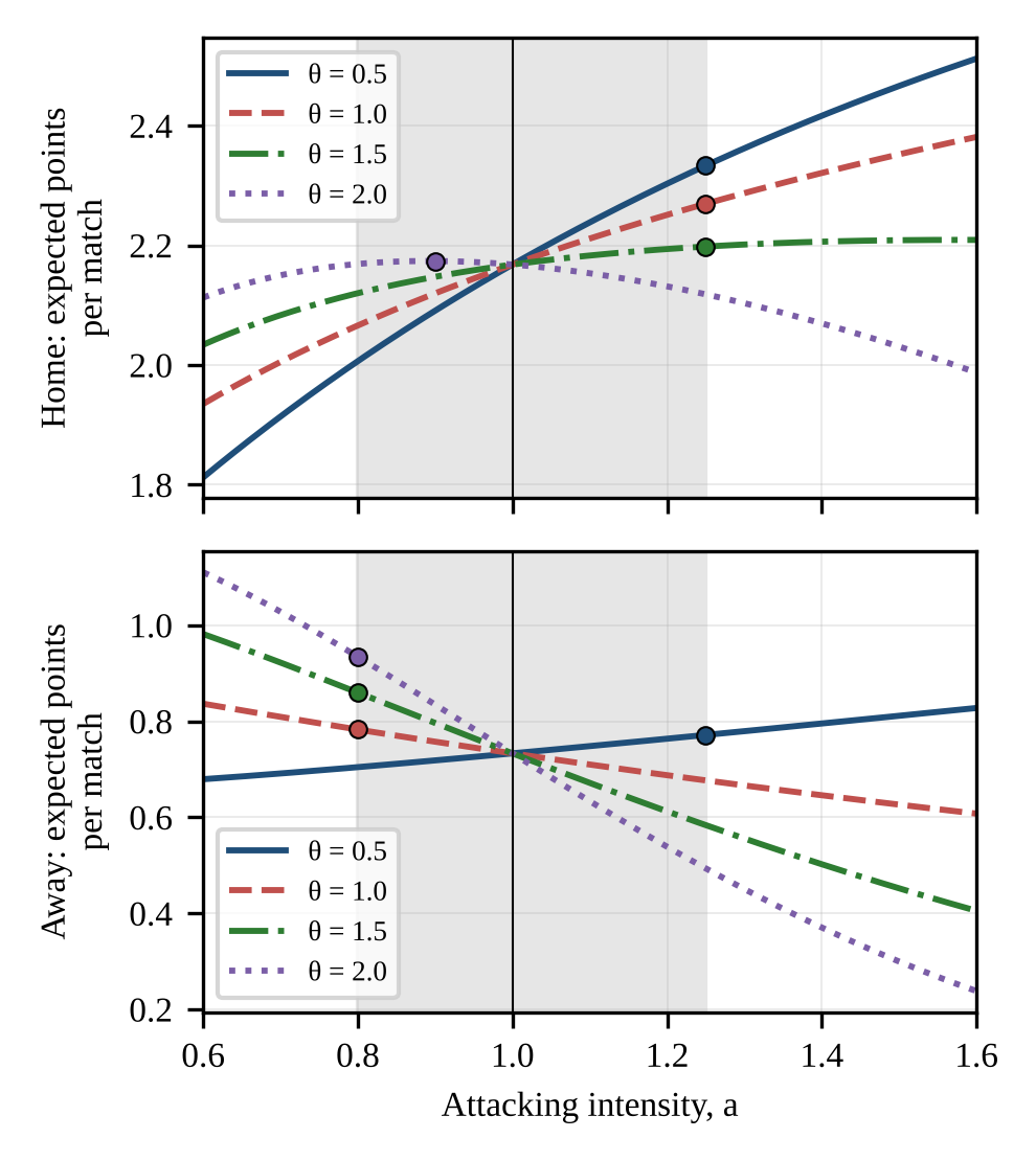
At home, a more attacking approach raises expected points for θ = 0.5 and 1.0, with credible intervals for the gain that exclude zero (Table 6). For θ = 1.5 and 2.0 the gains are near zero and their intervals include it. Away from home, a more cautious approach raises expected points for θ = 1.5 and 2.0, again with intervals excluding zero, and is favoured but uncertain at θ = 1.0 (P(gain > 0) = 0.92). In seven of the eight cases the best a sits on a search bound, so it shows direction only, and the home gain of +0.006 at θ = 2.0 is negligible. Figure 1 shows the underlying curves at the fitted rates.

Venue	θ	Best a	Gain, median (95% credible interval)	P(gain > 0)	P(best a > 1)
Home	0.5	1.25†	+0.160 (+0.119 to +0.176)	1.00	1.00
Home	1.0	1.25†	+0.099 (+0.032 to +0.117)	1.00	1.00
Home	1.5	1.25†	+0.029 (−0.086 to +0.081)	0.72	0.77
Home	2.0	0.85	+0.006 (−0.051 to +0.104)	0.55	0.31
Away	0.5	1.25†	+0.040 (−0.010 to +0.125)	0.91	0.89
Away	1.0	0.80†	+0.049 (−0.024 to +0.071)	0.92	0.07
Away	1.5	0.80†	+0.126 (+0.048 to +0.151)	1.00	0.00
Away	2.0	0.80†	+0.197 (+0.111 to +0.239)	1.00	0.00

Note: † On a search bound (0.80 or 1.25). Baseline expected points: 2.168 (home), 0.733 (away).

The bound-free summary tells the same story. Expected points rise with attacking intensity at home whenever θ is below θ₀ = 1.81 (95% credible interval 1.16 to 3.12), and away whenever θ is below θ₀ = 0.70 (0.40 to 1.13). The away interval spans 1, so whether a trade-off of θ = 1 favours caution away is itself uncertain. With negative binomial away scoring, θ₀ is 0.68 (0.43 to 0.86) and the gains for θ = 0.5, 1.0, 1.5 and 2.0 are +0.027, +0.044, +0.109 and +0.171, leaving the direction unchanged. Over ten matches the largest gains are about 1.6 points at home (θ = 0.5) and 2.0 points away (θ = 2.0). These are scenario results, not estimates of Solution FC’s true tactical optimum, since θ is assumed and the functional form is stylised.

3.5Counterfactual comparisons

Lifting away scoring to the home rate would add 0.86 expected points per away match (95% credible interval 0.20 to 1.49). Lowering away conceding to the home rate would add 0.48 (−0.09 to 1.03). Doing both reproduces the full gap of 1.40 (Table 7). The posterior probability that the scoring change is worth more than the conceding change is 0.78, which is only weak evidence that scoring explains more of the gap than conceding.

Change	Median	95% credible interval	P(> 0)
Away scoring rate set to home rate	+0.86	+0.20 to +1.49	0.995
Away conceding rate set to home rate	+0.48	−0.09 to +1.03	0.950
Both	+1.40	+0.51 to +2.08	0.998

3.6Simulated season outcomes

Simulated seasons centre on the observed total but spread widely (Table 8). Under the Poisson model the mean is 29.0 points with a 95% interval of 17 to 42, so the 29 points earned are one of many plausible results. The chances of reaching at least 29, 35 and 40 points are 0.535, 0.196 and 0.053. Negative binomial away scoring lowers the mean to 28.4 points (95% interval 16 to 40), with corresponding probabilities of 0.500, 0.159 and 0.037.

Outcome	Poisson	Negative binomial away scoring
Home (10 matches)	21.4 (11 to 30)	21.4 (11 to 30)
Away (10 matches)	7.7 (1 to 17)	7.1 (1 to 16)
Season (20 matches)	29.0 (17 to 42)	28.4 (16 to 40)

4Discussion

4.1Main findings

Solution FC’s season shows a large but uncertain venue effect. With a weak prior the Poisson model puts the home–away gap at 1.40 expected points per match (0.51 to 2.08); with rates partly pooled towards the club’s overall means it falls to 0.74 (0.05 to 1.36). The defensible statement is that the gap is probably positive and probably lies between roughly 0.7 and 1.4 points per match, not that it equals 1.40.

Away scoring seems to explain more of the gap than away conceding: raising each to its home level would add 0.86 and 0.48 points respectively. The credible intervals overlap, though, and the probability that scoring matters more is only 0.78. Seven of the ten away matches ended without a Solution FC goal, and the dispersion test hints, without settling the matter, that this exceeds what Poisson variation at the average away rate would produce.

The unbeaten home record deserves caution. Six wins and four draws look striking, yet the model assigns about a 22% chance to a home season without defeat, and the posterior predictive checks do not mark it as unusual. Chance may well account for part of it.

4.2What the scenario analysis shows

The scenario results are conditional and illustrative. At home, extra attack pays unless the defensive cost is steep (θ below about 1.8). Away, caution pays unless the cost of attacking is very mild (θ above about 0.7). Even so, the gains are small, at most about two points over ten matches, their intervals often include zero, and seven of the eight best values sit on the search bounds. The analysis shows how the decision depends on θ; it is not advice to change tactics. Coaching staff would have to judge the trade-off themselves or estimate it from shot and chance data. The simulations add a reminder of how much chance shapes a single season: 29 points is the typical outcome for this scoring profile, and a 40-point season turns up in roughly 5% of simulated seasons.

4.3Relation to earlier work

At league level, Pollard and Gómez found that Nigerian home teams took about 87% of league points over 2006–2012, the highest among 157 leagues [2]. Solution FC took 76% of its points (22 of 29) at home. The two figures differ in competition, period and measure, so the comparison should not be pressed. The club’s gap of 1.40 points exceeds the 0.39 points per game McCarrick et al. report for matches before the restrictions [3], but that comparison is also not like-for-like, and the shrinkage analysis suggests the excess is partly an artefact of picking an extreme club.

The mixed picture across leagues in [4] is a reminder that home advantage depends on context, which is the case for modelling a club’s own rates. The Bayesian approach follows the spirit of [9], scaled down to one club and one season, and the negative binomial check echoes the observation in [11] that count margins can be overdispersed relative to Poisson. The data cannot say why away results are weaker. Crowd support, travel, pitch familiarity and refereeing are often cited as sources of home advantage [3, 18], but none can be isolated here.

4.4Limitations and future work

One club, one season. Twenty matches produce wide intervals, and a single-club design cannot support league-wide inference. The natural extension is a hierarchical Poisson or Dixon–Coles-type model for all clubs in Conference B or the whole NNL, allowing pooling across clubs, adjustment for opponent strength and a proper test of home advantage. Only Solution FC’s results were available here.

Selection and regression to the mean. The club was chosen partly for its extreme split, so weak-prior estimates probably overstate the gap. The shrinkage analysis helps only in part, because its prior is centred on the club’s own mean rather than on other clubs.

No opponent adjustment. Opponents and dates are listed in Table 9 but not modelled, so a harder away schedule could explain some of the gap.

Independence and overdispersion. Scored and conceded goals are assumed independent (observed correlation −0.01). Away-scoring overdispersion is suggestive but does not survive a Bonferroni correction. The main analysis keeps the Poisson model, and the negative binomial check changes some figures slightly but not the conclusions.

Assumed trade-off. The form and strength of the attack–defence trade-off are assumed and the search range is bounded, so the scenario analysis is illustrative.

Constant rates. Scoring and conceding rates are assumed fixed across the season. Future work could add earlier seasons where reliable records exist, extend the analysis to every club in the conference, adjust for opponent strength, let rates vary within the season, and estimate θ from within-match indicators such as shots and goals conceded.

5Conclusion

Solution FC’s 2024/25 NNL points were driven mainly by a wide gap between home and away scoring and conceding rates. A Poisson model gives expected points of 2.17 per home match and 0.73 per away match, a difference of 1.40 (95% credible interval 0.51 to 2.08) that drops to 0.74 (0.05 to 1.36) once the rates are partly pooled towards the club’s overall means. The data do not clearly contradict the Poisson model, although away scoring is overdispersed; the negative binomial check leaves the conclusions largely intact. Venue-specific rates predicted held-out matches better than pooled rates on average, but not decisively.

The scenario analysis shows that the preferred attacking intensity hinges on an assumed trade-off. More attack pays at home unless the trade-off is steep (θ below about 1.8), and caution pays away unless it is very mild (θ above about 0.7). The gains are small, uncertain and often on the search bounds, so they are illustrative only. The study covers one club and one season. It does give a reproducible way to report club-level home and away performance together with its uncertainty, and its logical successor is a hierarchical model covering every club in the conference.

Appendix

Match records analysed

Solution FC’s goals are listed first in Table 9; “Day” is the matchday. The club had no fixture on matchdays 3 and 20 (see Design, season format and data, and Table 10).

Day	Date	Venue	Opponent	Score	Pts
1	6 Dec 2024	Home	Rovers FC	1–1	1
2	16 Dec 2024	Away	Sporting Lagos FC	0–4	0
4	4 Jan 2025	Home	First Bank FC	2–0	3
5	11 Jan 2025	Away	Gateway United FC	3–2	3
6	18 Jan 2025	Home	Kun Khalifat FC	2–0	3
7	25 Jan 2025	Away	Abakaliki FC	0–0	1
8	1 Feb 2025	Home	Madiba FC	4–1	3
9	8 Feb 2025	Away	ABS FC	0–1	0
10	15 Feb 2025	Home	God’s will Akpabio FC	1–0	3
11	1 Mar 2025	Away	Osun United FC	0–1	0
12	6 Apr 2025	Home	Osun United FC	1–1	1
13	11 Apr 2025	Away	God’s will Akpabio FC	1–4	0
14	20 Apr 2025	Home	ABS FC	3–0	3
15	25 Apr 2025	Away	Madiba FC	0–1	0
16	7 May 2025	Home	Abakaliki FC	1–0	3
17	10 May 2025	Away	Kun Khalifat FC	0–1	0
18	18 May 2025	Home	Gateway United FC	2–2	1
19	23 May 2025	Away	First Bank FC	0–1	0
21	8 Jun 2025	Home	Sporting Lagos FC	3–3	1
22	14 Jun 2025	Away	Rovers FC	3–1	3

Fixture structure

Each opponent appears once per half, with the venue reversed in the second half (Table 10). The second-half matchday equals 23 minus the first-half matchday, so the idle matchdays 3 and 20 also form a mirrored pair.

Opponent	First half	Second half
Rovers FC	Matchday 1, home	Matchday 22, away
Sporting Lagos FC	Matchday 2, away	Matchday 21, home
First Bank FC	Matchday 4, home	Matchday 19, away
Gateway United FC	Matchday 5, away	Matchday 18, home
Kun Khalifat FC	Matchday 6, home	Matchday 17, away
Abakaliki FC	Matchday 7, away	Matchday 16, home
Madiba FC	Matchday 8, home	Matchday 15, away
ABS FC	Matchday 9, away	Matchday 14, home
God’s will Akpabio FC	Matchday 10, home	Matchday 13, away
Osun United FC	Matchday 11, away	Matchday 12, home
No fixture (idle)	Matchday 3	Matchday 20

Acknowledgment

The authors gratefully acknowledge the contributions of all individuals and institutions whose support, guidance, and resources contributed to the successful completion of this research. Special appreciation is extended to those who provided relevant information and materials that supported the study. The author also appreciates the scholarly contributions of researchers whose published works informed the theoretical and methodological foundations of this study.

Any errors or shortcomings that remain in the manuscript are the sole responsibility of the authors.

Conflict of Interest: The authors declare that there are no conflicts of interest that could have influenced the research, its analysis, or the preparation of this manuscript.

Funding: This research received no specific grant from any funding agency in the public, commercial, or not-for-profit sectors.

References

1. [1]Pollard R, Pollard G. Long-term trends in home advantage in professional team sports in North America and England (1876–2003). J Sports Sci. 2005;23(4):337–350. https://doi.org/10.1080/02640410400021559
2. [2]Pollard R, Gómez MA. Components of home advantage in 157 national soccer leagues worldwide. Int J Sport Exerc Psychol. 2014;12(3):218–233. https://doi.org/10.1080/1612197X.2014.888245
3. [3]McCarrick D, Bilalic M, Neave N, Wolfson S. Home advantage during the COVID-19 pandemic: Analyses of European football leagues. Psychol Sport Exerc. 2021;56:102013. https://doi.org/10.1016/j.psychsport.2021.102013
4. [4]Benz LS, Lopez MJ. Estimating the change in soccer’s home advantage during the Covid-19 pandemic using bivariate Poisson regression. AStA Adv Stat Anal. 2023;107(1–2):205–232. https://doi.org/10.1007/s10182-021-00413-9
5. [5]Wang S, Qin Y. The impact of crowd effects on home advantage of football matches during the COVID-19 pandemic: A systematic review. PLoS One. 2023;18(11):e0289899. https://doi.org/10.1371/journal.pone.0289899
6. [6]Maher MJ. Modelling association football scores. Stat Neerl. 1982;36(3):109–118. https://doi.org/10.1111/j.1467-9574.1982.tb00782.x
7. [7]Dixon MJ, Coles SG. Modelling association football scores and inefficiencies in the football betting market. J R Stat Soc Ser C Appl Stat. 1997;46(2):265–280. https://doi.org/10.1111/1467-9876.00065
8. [8]Karlis D, Ntzoufras I. Analysis of sports data by using bivariate Poisson models. J R Stat Soc Ser D Statistician. 2003;52(3):381–393. https://doi.org/10.1111/1467-9884.00366
9. [9]Lee J, Kim J, Kim H, Lee JS. A Bayesian approach to predict football matches with changed home advantage in spectator-free matches after the COVID-19 break. Entropy. 2022;24(3):366. https://doi.org/10.3390/e24030366
10. [10]Ribeiro GG, da Costa LCC, Ferreira PH, do Nascimento DC. A Bayesian approach to predict performance in football: A case study. Front Sports Act Living. 2025;7:1486928. https://doi.org/10.3389/fspor.2025.1486928
11. [11]Michels R, Ötting M, Karlis D. Extending the Dixon and Coles model: An application to women’s football data. arXiv:2307.02139 [Preprint]. 2023. https://arxiv.org/abs/2307.02139
12. [12]Beal R, Chalkiadakis G, Norman TJ, Ramchurn SD. Optimising game tactics for football. In: Proceedings of the 19th International Conference on Autonomous Agents and Multiagent Systems (AAMAS). 2020. https://arxiv.org/abs/2003.10294
13. [13]Solution FC Media. Solution FC Southern Conference B stats for the 2024/2025 NNL season [club season statistics and results summary]. 2025.
14. [14]Flashscore (incl. Flashfootball). NNL 2024/2025: Results and standings [data platform]. Nigeria > NNL. n.d.
15. [15]Soccerway. Nigeria NNL 2024/2025: Standings and results [data platform]. n.d. https://www.soccerway.com/nigeria/nnl/
16. [16]Nigeria National League. Nigeria National League [official Facebook page]. Meta Platforms. n.d.
17. [17]Arise News. Nigeria National 2024/2025 League to kick off November 30 with opening matches across all conferences. 2024. https://arise.tv/nigeria-national-2024-2025-league-to-kick-off-november-30-with-opening-matches-across-all-conferences
18. [18]Sedeaud A, De Larochelambert Q, Schipman J, Toussaint JF. The COVID-19 pandemic impact on away and home victories in soccer and rugby union. Front Sports Act Living. 2021;3:695922. https://doi.org/10.3389/fspor.2021.695922