Explainable AI for Imbalanced Credit Card Fraud Detection: A Comparative Study

1Introduction

Electronic payment systems process large volumes of transactions, while confirmed fraud is comparatively uncommon. This imbalance creates a misleading evaluation problem: a classifier that labels every transaction as legitimate can attain high accuracy without detecting any fraud. Consequently, accuracy should not be the primary measure of a fraud detector's usefulness [1], [3].

Two related challenges motivate this study. First, model performance depends on how the training process addresses the scarcity of fraud examples. Second, analysts need information about why a transaction receives a high-risk score. This work therefore compares four classification algorithms under three imbalance-handling conditions and examines both predictive performance and model explanations.

The study has three objectives:

1. 1. Compare Logistic Regression, Decision Tree, Random Forest, and XGBoost with no imbalance adjustment, SMOTE, or class weighting on the ULB Credit Card Fraud Detection dataset.
2. 2. Select one of the twelve configurations using an explicit eligibility gate and a weighted ranking rule that excludes accuracy.
3. 3. Explain predictions from the selected model with SHAP [5] and demonstrate the model in a Flask-based research prototype.

The evaluation separates training and test data before fitting preprocessing steps or applying SMOTE. Performance is reported using Precision, Recall, F1-score, ROC-AUC, and PR-AUC. The paper's results support selecting XGBoost with class weighting over the simpler models, but provide less decisive evidence of superiority over Random Forest. The prototype is intended for research demonstration rather than operational payment decisions.

2Related work

Class imbalance is a longstanding issue in fraud detection [1]. SMOTE addresses minority-class scarcity by generating synthetic examples from neighboring minority observations [2]. Cost-sensitive learning offers another approach by assigning greater training importance to costly errors, such as missed fraud. These approaches alter the learning process in different ways, so their effects may depend on the classifier.

Fraud-detection evaluation also needs to reflect the rare-event setting. Precision-recall analysis focuses on the trade-off between identifying positive cases and the reliability of positive alerts; it can therefore be more informative than ROC analysis when the negative class is much larger [3]. Prior work on credit-card fraud detection has emphasized realistic evaluation procedures that account for how alerts are generated and investigated [1].

Logistic Regression provides a relatively transparent baseline, while tree ensembles such as Random Forest and XGBoost can represent more complex relationships in tabular data [4]. SHAP assigns feature contributions to individual predictions using Shapley-value principles and provides a unified framework for interpreting model output [5]. This study brings together imbalance handling, rare-event evaluation, and post-hoc explanation in one controlled comparison.

3Problem definition and dataset

Let each transaction be represented by a feature vector x_i ∈ ℝ^d, with label y_i ∈ {0, 1}, where 0 denotes a legitimate transaction and 1 denotes fraud. The objective is to estimate a score f(x) representing the estimated probability of fraud. A transaction is classified as positive when its score meets or exceeds a decision threshold τ.

3.1Dataset description

The ULB Credit Card Fraud Detection dataset, distributed through Kaggle, contains 284,807 European cardholder transactions recorded over two days (Table 1). Of these, 284,315 are legitimate and 492 are fraudulent, corresponding to a fraud prevalence of 0.173% (Figure 1) and an approximate legitimate-to-fraud ratio of 578:1. The 30 predictors comprise Time, Amount, and 28 anonymized principal-component variables, V1–V28. No additional attributes, such as merchant category or location, were added.

Quantity	Value
Transactions (raw file)	284,807
Legitimate / fraudulent	284,315 / 492
Features (Time, Amount, V1–V28)	30
Missing values / exact duplicates	0 / 1,081
Rows after duplicate removal (fraud)	283,726 (473)
Training rows (fraud)	226,980 (378)
Test rows (fraud)	56,746 (95)
Training rows after SMOTE	453,204

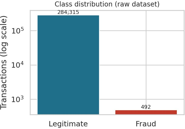
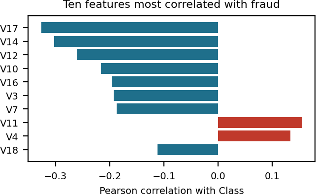
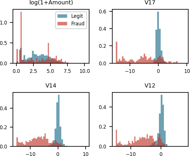
The observed fraud rate varies across six-hour time blocks, from 0.075% in the 30–36-hour block to 0.595% in the 24–30-hour block (Table 2). The Time variable measures elapsed seconds from the beginning of the dataset; it is not a clock-time field, so these differences should not be interpreted as time-of-day patterns. The largest reported linear correlations with the fraud label are V17 (−0.327), V14 (−0.302), and V12 (−0.261) (Figure 2); Figure 3 compares the class-conditional distributions of Amount and three of these features. These relatively modest correlations indicate that no single feature provides a simple linear separation of the classes.

Block	Transactions	Frauds	Rate (%)
0–6 h	12,340	55	0.446
6–12 h	35,061	91	0.260
12–18 h	46,850	71	0.152
18–24 h	50,535	64	0.127
24–30 h	11,594	69	0.595
30–36 h	35,851	27	0.075
36–42 h	49,585	63	0.127
42–48 h	42,991	52	0.121

An interquartile-range screen identified substantial numbers of extreme observations, including 13.8% for V27, 11.2% for Amount, 10.7% for V28, and 9.8% for V20. These records were retained because extreme values may carry useful fraud information and removing them would discard a material part of the data.

4Methods

4.1Data preparation and split

The raw file contained no missing values and 1,081 exact duplicate rows. Exact duplicates were removed before splitting to prevent identical records from appearing in both training and test partitions. The resulting 283,726 records were divided using a stratified 80/20 split with random seed 42. The training partition contained 226,980 transactions, including 378 fraud cases; the test partition contained 56,746 transactions, including 95 fraud cases (Table 1).

Time and Amount were transformed with a robust scaler. The medians and interquartile ranges were estimated using the training data only, then applied to both partitions. V1–V28 were not rescaled. Outliers identified by the 1.5 × IQR rule were retained.

5Imbalance-handling conditions

Each algorithm was evaluated under three conditions: (1) no imbalance adjustment, (2) SMOTE oversampling, and (3) class weighting. SMOTE was applied only after the train-test split and only to the training partition. It increased the training-set size from 226,980 to 453,204 records. The test data were neither resampled nor otherwise altered, preserving their observed class distribution. Class weighting increased the influence of fraud examples during model fitting; the unadjusted condition used unit weights.

6Classification algorithms

Logistic Regression estimates fraud probabilities through a logistic function and fits its parameters using regularized log-loss. Class weights can be incorporated into the loss. A Decision Tree recursively partitions observations, selecting splits that reduce node impurity, measured here with the Gini criterion.

Random Forest combines predictions from multiple decision trees trained on bootstrap samples and randomized feature subsets. XGBoost builds trees sequentially, with each new tree contributing to an additive model optimized using a regularized loss [4]. The same fixed hyperparameter settings were used for each algorithm across imbalance conditions; no hyperparameter search was performed.

7Evaluation measures

At threshold τ, the confusion matrix contains true positives (TP), false positives (FP), true negatives (TN), and false negatives (FN). Precision measures the proportion of flagged transactions that are fraudulent, while Recall measures the proportion of fraud cases detected. The F1-score is the harmonic mean of Precision and Recall. ROC-AUC summarizes discrimination across thresholds using the true-positive and false-positive rates. PR-AUC, computed as average precision, summarizes the precision-recall relationship across thresholds.

Because legitimate transactions dominate this dataset, ROC-AUC is reported alongside PR-AUC rather than used alone [3]. Accuracy is included for context but is not part of the model-selection rule.

8Model-selection rule

Selection proceeds in two stages. A configuration is eligible only if its test-set Recall is at least 0.60 and its Precision is at least 0.30. Eligible configurations are ranked using the following score:

where R is Recall, P is Precision, F₁ is the F1-score, and AP is PR-AUC. Ties are resolved in favor of the larger PR-AUC. The weights were intended to reflect the study's priority of detecting fraud, but the source manuscript does not provide their values. The weights must be supplied before this selection rule can be reproduced.

9Explainability

SHAP represents a prediction as a baseline value plus contributions from the input features [5]. Positive contributions increase the model output relative to the baseline, while negative contributions decrease it. TreeSHAP was used for tree-based models, and a linear explainer was used for Logistic Regression. Explanations were calculated for 2,000 test transactions. Contributions for XGBoost and Logistic Regression are reported in log-odds; contributions for the scikit-learn tree models are reported as changes in probability.

10Risk bands and decision threshold

The prototype maps predicted fraud probabilities to LOW, MEDIUM, or HIGH risk using configurable research thresholds. Those threshold definitions are missing from the supplied manuscript and must be restored from the implementation or original draft. They should not be inferred. The binary prediction threshold used for the reported evaluation was fixed at τ = 0.5.

11Experimental setup

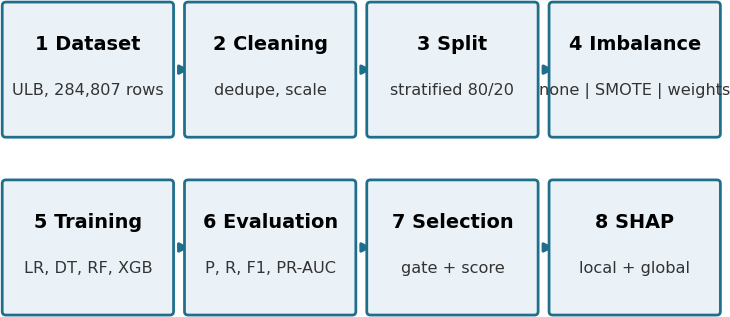
All twelve combinations of four algorithms and three imbalance conditions used the same data split and training-only scaling procedure. The implementations used scikit-learn, imbalanced-learn, XGBoost, and SHAP. The recorded environment was Python 3.12, scikit-learn 1.8, imbalanced-learn 0.14, XGBoost 3.4, and SHAP 0.52, running on a CPU-only machine. The fixed hyperparameters are listed in Table 3, and Figure 4 shows the experimental pipeline. Random processes used seed 42. Two scripts were used to generate the experiments and results. Each model was evaluated once on the held-out test set, which was not used to fit preprocessing, resample observations, tune hyperparameters, or select the classification threshold.

Algorithm	Hyperparameters
Logistic Regression	L2 penalty, C=1, lbfgs, max_iter=2000
Decision Tree	Gini, max_depth=8, min_samples_leaf=10
Random Forest	100 trees, max_depth=12, min_samples_leaf=2
XGBoost	300 trees, depth=6, learning_rate=.1, subsample=.8, colsample_bytree=.8, hist, AUCPR
SMOTE	k=5, training partition only
All	seed=42; threshold τ=.5

12Results

12.1Comparative performance and selection

Performance varied across the twelve configurations (Table 4). Recall changed substantially, whereas ROC-AUC remained high across models; this illustrates why ROC-AUC alone does not describe performance under severe class imbalance. The effect of SMOTE and class weighting also depended on the algorithm. In some configurations, Recall increased at the expense of Precision, particularly for Logistic Regression and the Decision Tree. Random Forest and XGBoost were comparatively stable across the tested conditions. Figures 5 and 6 show the precision-recall and ROC curves for the class-weighted configurations, and Figures 7 and 8 the precision-recall curves without imbalance handling and with SMOTE.

Model	Technique	Prec.	Recall	F1	ROC-AUC	PR-AUC
Logistic Regression	No handling	.862	.589	.700	.958	.695
Decision Tree	No handling	.872	.716	.786	.913	.753
Random Forest	No handling	.972	.737	.838	.972	.795
XGBoost	No handling	.946	.737	.828	.976	.812
Logistic Regression	SMOTE	.054	.874	.101	.960	.673
Decision Tree	SMOTE	.103	.842	.183	.893	.485
Random Forest	SMOTE	.710	.800	.752	.979	.796
XGBoost	SMOTE	.760	.800	.779	.968	.810
Logistic Regression	Class weight	.056	.874	.106	.966	.672
Decision Tree	Class weight	.138	.800	.236	.907	.496
Random Forest	Class weight	.886	.737	.805	.971	.807
XGBoost	Class weight	.974	.789	.872	.973	.823

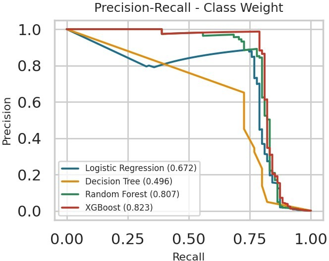
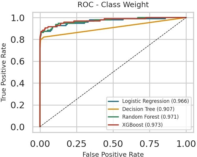
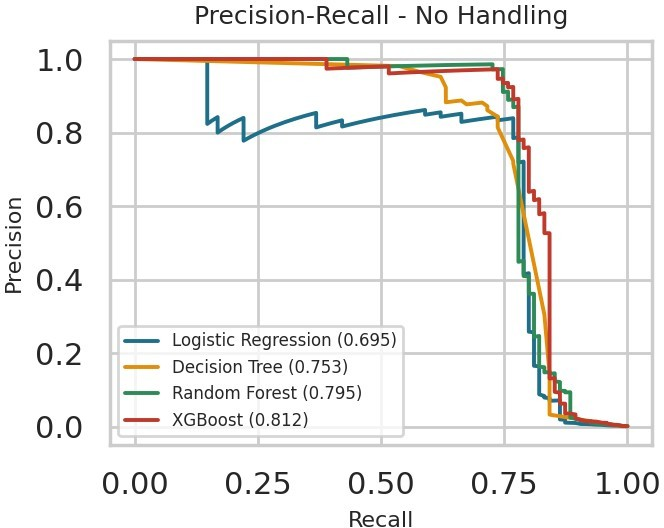
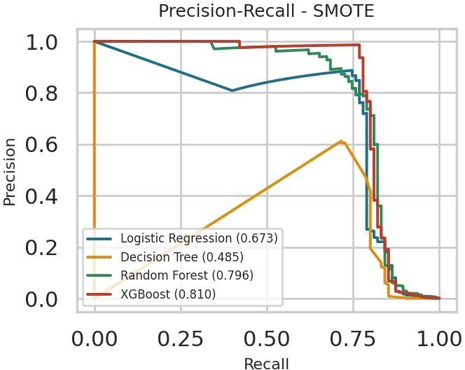
The reported top three composite scores were XGBoost with class weighting (0.860), Random Forest without imbalance handling (0.830), and XGBoost without imbalance handling (0.826). The selected configuration, XGBoost with class weighting, achieved Recall 0.789, Precision 0.974, F1-score 0.872, and PR-AUC 0.823. These values correspond to detecting most of the fraud cases while maintaining high precision on the test set. Table 5 gives the mean metrics for each imbalance-handling technique, Table 6 the changes relative to no handling, and Figure 9 the confusion matrix of the selected model.

Technique	Precision	Recall	F1	PR-AUC
No handling	.913	.695	.788	.764
SMOTE	.407	.829	.454	.691
Class weight	.514	.800	.505	.699

Model	Technique	ΔRecall	ΔPrecision	ΔPR-AUC
Logistic Regression	SMOTE	+.284	−.808	−.022
Logistic Regression	Class weight	+.284	−.805	−.023
Decision Tree	SMOTE	+.126	−.769	−.267
Decision Tree	Class weight	+.084	−.734	−.257
Random Forest	SMOTE	+.063	−.262	+.001
Random Forest	Class weight	+.000	−.086	+.012
XGBoost	SMOTE	+.063	−.186	−.002
XGBoost	Class weight	+.053	+.028	+.011

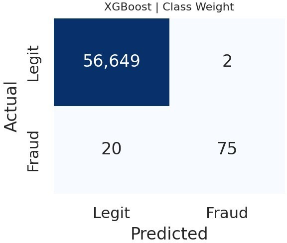
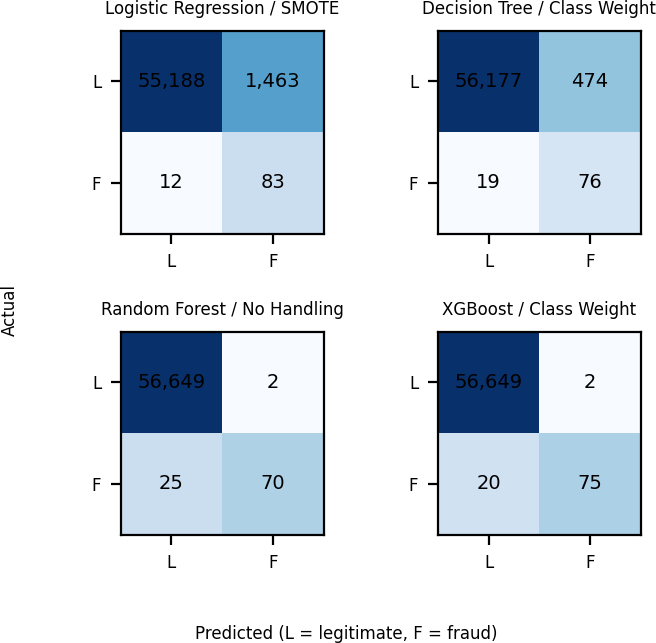
A classifier that labels every test record as legitimate would attain accuracy 0.9983 while detecting no fraud. The selected model's reported accuracy was 0.9996, only 0.0013 higher (Table 7, Figure 10). Some configurations performed below the trivial classifier's accuracy despite detecting fraud. These comparisons show why accuracy was excluded from the selection rule.

Model	Technique	TP	FN	FP	Accuracy
Logistic Regression	No handling	56	39	9	.9992
Decision Tree	No handling	68	27	10	.9993
Random Forest	No handling	70	25	2	.9995
XGBoost	No handling	70	25	4	.9995
Logistic Regression	SMOTE	83	12	1,463	.9740
Decision Tree	SMOTE	80	15	699	.9874
Random Forest	SMOTE	76	19	31	.9991
XGBoost	SMOTE	76	19	24	.9992
Logistic Regression	Class weight	83	12	1,393	.9752
Decision Tree	Class weight	76	19	474	.9913
Random Forest	Class weight	70	25	9	.9994
XGBoost	Class weight	75	20	2	.9996

13Uncertainty and comparison with other algorithms

The test partition contained only 95 fraud cases, so performance estimates are uncertain. The study used 500 bootstrap resamples of the test transactions to calculate percentile confidence intervals for the best-performing configuration of each algorithm. For the selected XGBoost model, the reported Recall interval was 0.71–0.87 (Table 8). Training times are given in Table 9.

Model	Recall	Precision	PR-AUC
Logistic Regression (No Handling)	0.589 [0.49,0.68]	0.862 [0.78,0.94]	0.695 [0.60,0.79]
Decision Tree (No Handling)	0.716 [0.62,0.80]	0.872 [0.79,0.94]	0.753 [0.67,0.84]
Random Forest (No Handling)	0.737 [0.65,0.82]	0.972 [0.93,1.00]	0.795 [0.72,0.87]
XGBoost (Class Weight)	0.789 [0.71,0.87]	0.974 [0.93,1.00]	0.823 [0.76,0.89]

Model	No handling	SMOTE	Class weight
Logistic Regression	0.5	2.4	1.0
Decision Tree	10.0	17.4	8.8
Random Forest	142.6	272.9	110.8
XGBoost	9.5	18.5	10.2

Paired bootstrap comparisons on the same resamples (Table 10) found that XGBoost performed better than Logistic Regression and the Decision Tree, with confidence intervals for the differences excluding zero. The comparison with Random Forest was less conclusive. The mean PR-AUC difference was +0.029, but its interval included zero. The F1-score difference was +0.036, with a reported interval of +0.007 to +0.070. Taken together, these estimates support an advantage over the simpler models but do not establish a robust overall advantage over Random Forest. More fraud cases, repeated splits, or repeated cross-validation would be needed to resolve the close comparison.

Comparison	ΔPR-AUC	ΔF1	XGB better (PR-AUC)
vs. Logistic Regression	+.128 [+.057,+.204]	+.176 [+.109,+.246]	100.0%
vs. Decision Tree	+.069 [+.022,+.120]	+.088 [+.049,+.132]	99.8%
vs. Random Forest	+.029 [−.002,+.060]	+.036 [+.007,+.070]	97.0%

14Threshold analysis and error patterns

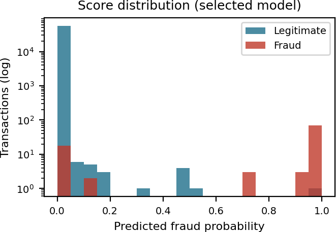
The primary evaluation used a fixed threshold of 0.5. Across thresholds from 0.2 to 0.7, the reported Recall remained 0.789, while the number of false alarms changed from seven to one (Table 11, Figure 11). At a threshold of 0.1, two additional fraud cases were detected at the cost of 13 additional false alarms. The reported score distribution was strongly concentrated near zero or one, consistent with the limited change in Recall over the middle threshold range.

τ	Precision	Recall	F1	TP	FP	FN
.1	.837	.811	.824	77	15	18
.2	.915	.789	.847	75	7	20
.3	.915	.789	.847	75	7	20
.4	.926	.789	.852	75	6	20
.5	.974	.789	.872	75	2	20
.6	.987	.789	.877	75	1	20
.7	.987	.789	.877	75	1	20
.8	.986	.758	.857	72	1	23
.9	.986	.758	.857	72	1	23

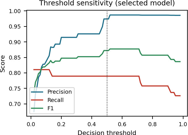
The 20 missed fraud cases were not generally close to the decision boundary: their median predicted probability was 0.0001, 17 had probabilities below 0.01, and two exceeded 0.10. This suggests that modest threshold reductions would recover few of these cases using the available features (Figure 12). The source manuscript also reports two false alarms with probabilities of 0.512 and 1.000. This count should be reconciled with the threshold analysis, which reports between one and seven false alarms across thresholds 0.2–0.7; the supplied material does not clearly identify which threshold and table produced the count of two.

Under the reported risk bands, the HIGH group contained 75 fraud cases among 76 flagged transactions, for a Precision of 98.7% (Table 12). The LOW group had a fraud rate of 0.035%, compared with 0.167% in the full test set, but still contained 20 fraud cases. The MEDIUM group contained only five transactions. Thus, a LOW label did not guarantee legitimacy, and the near-empty MEDIUM category had limited practical value for this model and dataset.

Risk level	Transactions	Fraud	Legitimate
LOW	56,665	20	56,645
MEDIUM	5	0	5
HIGH	76	75	1

15SHAP explanations

For the selected XGBoost model, the five features with the largest mean absolute SHAP contributions were V14, V4, V12, V10, and V11. The next five were V3, V8, V19, V1, and V28 (Figure 13). Three of the leading five features—V14, V12, and V10—were also among the four variables with the strongest reported linear correlations with the label. V4 and V11 had weaker linear correlations, suggesting that the model's reliance on features is not fully captured by one-feature-at-a-time linear association.

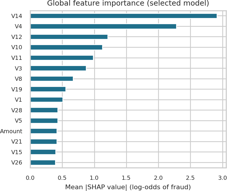
The V-features are anonymized principal components. SHAP therefore indicates how these model inputs influenced predictions but cannot identify the underlying transaction characteristics or establish causal explanations. For an individual transaction, the prototype displays the largest positive and negative contributions to help users inspect the score.

16Flask prototype

The experiment code and web application are separated. The training pipeline writes model metrics, figures, and the selected model to files; the Flask application and research dashboard read those saved outputs rather than embedding reported results directly in the application (Figure 14).

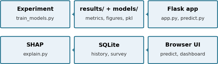
The prediction interface accepts Time, Amount, and V1–V28 and checks submitted values against ranges observed in the dataset. It can also load labelled examples from the held-out test set, allowing demonstrations without personal transaction data. For each input, the application displays a fraud probability, risk band, binary prediction, and leading SHAP contributions. It also identifies the V-variables as anonymized features.

The application does not request payment-card numbers, CVV codes, one-time passwords, PINs, or account passwords. The described implementation uses CSRF protection, can restrict stored-data export with an administrator token, and stores prediction history locally in SQLite. An optional survey module collects no personal information, and survey data are not used to train or evaluate the model. Because this is a research prototype, outputs are labelled as “Potentially Fraudulent” or “Likely Legitimate,” rather than as final decisions.

17Limitations

Dataset coverage. The dataset contains anonymized features and only two days of European card transactions. It cannot represent all regions, seasonal patterns, or future fraud strategies. Because the principal components have no direct transaction-level interpretation, model explanations cannot readily be translated into operational causes.

Evaluation design. Results are based on one stratified random split and only 95 fraudulent test observations. Confidence intervals are consequently wide, and the comparison between XGBoost and Random Forest remains uncertain. A random split also disregards transaction chronology and may produce more optimistic estimates than evaluation on future transactions.

Model development. Hyperparameters were fixed rather than tuned. This provides a controlled comparison under the selected settings but may not reflect each algorithm's best attainable performance. SMOTE and class weighting can affect probability calibration, so the displayed scores and research risk bands should not be treated as calibrated operational risk estimates. The classification threshold was fixed at 0.5 rather than chosen from an explicit cost model. The composite-score weights are not available in the supplied manuscript, preventing exact reproduction of the ranking.

Deployment scope. The prototype does not provide streaming inference, concept-drift monitoring, or an investigator feedback loop. These are important capabilities for real-world fraud systems [1]. The application demonstrates a research workflow and should not be interpreted as a production-ready fraud-control service.

18Conclusion

This study compared four machine-learning algorithms under three approaches to class imbalance using a leakage-conscious split of the ULB credit-card dataset. The results show that imbalance handling interacts with the choice of algorithm: SMOTE and class weighting can improve Recall, but may also sharply reduce Precision in some configurations.

The stated selection procedure chose XGBoost with class weighting, which achieved Recall 0.789, Precision 0.974, F1-score 0.872, and PR-AUC 0.823. Bootstrap comparisons support its advantage over Logistic Regression and Decision Tree more strongly than its advantage over Random Forest. The limited number of test fraud cases and single split counsel against treating the ranking as definitive. SHAP explanations and a Flask prototype demonstrate how predictions can be presented for research, but anonymized inputs limit the real-world meaning of feature attributions.

Further work should report the missing composite-score weights and exact risk-band definitions, tune hyperparameters, use repeated and time-ordered validation, calibrate probabilities, and select thresholds using explicit operational costs. Evaluation on datasets with interpretable transaction attributes and additional cardholder history may help investigate the fraud cases missed by the current features.

References

1. [1]Dal Pozzolo A, Boracchi G, Caelen O, Alippi C, Bontempi G. Credit card fraud detection: A realistic modeling and a novel learning strategy. IEEE Trans Neural Netw Learn Syst. 2018;29(8):3784–3797. https://doi.org/10.1109/TNNLS.2017.2736643
2. [2]Chawla NV, Bowyer KW, Hall LO, Kegelmeyer WP. SMOTE: Synthetic minority over-sampling technique. J Artif Intell Res. 2002;16:321–357. https://doi.org/10.1613/jair.953
3. [3]Saito T, Rehmsmeier M. The precision-recall plot is more informative than the ROC plot when evaluating binary classifiers on imbalanced datasets. PLoS One. 2015;10(3):e0118432. https://doi.org/10.1371/journal.pone.0118432
4. [4]Chen T, Guestrin C. XGBoost: A scalable tree boosting system. In: Proc. 22nd ACM SIGKDD Int. Conf. Knowledge Discovery and Data Mining. 2016. p. 785–794. https://doi.org/10.1145/2939672.2939785
5. [5]Lundberg SM, Lee SI. A unified approach to interpreting model predictions. In: Advances in Neural Information Processing Systems 30 (NeurIPS). 2017. p. 4765–4774.