Real-Time Video Stabilization Using a Modified Optical Flow Algorithm

1Introduction

Video stabilization removes the jitter that camera motion adds to a video. The motion may come from an uneven surface, from a vibrating platform, or from an unsteady hand. Stabilization methods fall into two classes. Offline (post-processing) methods clean up a video after it has been recorded [1]. Online, or real-time, methods do the same work while the video is being recorded, with no manual step [2].

Online stabilization can be done mechanically, optically or digitally, and the choice depends on the application. Combining two of these often gives better results [3]. Mechanical stabilization uses gyroscopes and dampers to cancel unwanted global motion [3]. Optical stabilization shifts a lens group to compensate for the camera’s angular and translational movement [3], [4]. Digital video stabilization (DVS) needs no special equipment because it runs entirely in software.

DVS has three main steps: motion estimation, motion compensation and image warping [5]. Motion estimation measures the global motion between frames by tracking the displacement of well-defined static features [6]. Motion compensation removes the global motion and keeps the local motion, and removing the global motion is what stabilizes the video [6], [7]. Image warping then transforms each frame toward the desired camera path. It moves the frame by the same amount as the jitter, but in the opposite direction [8], [9].

A video contains both intentional motion, such as a pan, and unintentional motion, such as shake. Many heuristic methods have been developed to remove the unintentional global motion while preserving the intentional local motion. They are usually grouped by how they estimate motion. Early work used two-dimensional (2D) estimation, which models simple scenes without depth by estimating camera motion from consecutive frames and applying 2D transformations [10]. Three-dimensional (3D) estimation instead recovers the 3D position of feature points, and with it the structure of the scene and the camera motion between frames, usually through structure from motion (SFM) [11], [12].

More recently, optical flow has drawn much attention for stabilization. This paper presents a real-time stabilizer built on a modified optical flow algorithm and running on a Raspberry Pi. We test it on a purpose-built vibration rig and compare its output with unstabilized video of the same scene. [16] use the standard optical flow algorithm to stabilize video frames his approach did not consider shaky videos with rotational effect, also the author did not implement the algorithm on a hardware this paper modified his approach to stabilize shaky videos with rotational effect and also implement the algorithm on a Raspberry Pi microcomputer. Section 2 reviews related work, Section 3 describes the method and experimental setup, Section 4 presents the results, and Section 5 concludes.

2Related work

2.1Two-dimensional methods

Early stabilizers tracked features in the image plane and modeled the frame motion as a 2D transformation. Grundmann et al. [13] track feature points and use constrained L1 optimization to find a camera path made of constant, linear and parabolic segments, which removes the global motion. Goldstein and Fattal [14] track feature points and use them to compute fundamental matrices, then synthesize new frames by image-based warping. They rely on the geometric relation between points and epipolar lines to keep the tracked features in place. Liu et al. [15] track 2D feature points, divide the frame into a grid mesh and let the motion vary across it. The mesh is then used to warp and smooth the output while preserving local motion.

These 2D methods share one weakness. Their motion models, such as affine or homography transformations, cannot describe frame changes when the scene has large depth variation [16].

2.2Three-dimensional methods

Three-dimensional methods estimate where feature points lie in space and compute the camera pose in 3D, so the sparse 3D information can guide the synthesis of new frames. Liu et al. [11] use structure from motion to find the 3D positions of feature points, re-project them onto a smoothed camera path, and use the projections to control a content-preserving warp of the original frames.

The weak point is structure from motion itself. Methods built on it, such as [11], suffer from robustness and complexity problems, and the algorithm fails on videos with zooming, quick rotation or fast-moving objects.

2.3Methods that use extra sensors

Depth cameras and motion sensors opened another route. Karpenko et al. [4] model camera motion and rolling-shutter warping, calibrate a gyroscope automatically, and use its data to correct jitter. Liu et al. [16] use the depth information from a depth camera to estimate homographies for the scene and to separate global from local motion. Smith et al. [17] optimize over space and time to compute the relative poses between a virtual camera and a camera array, which reduces the acceleration of salient features in the virtual image plane. The cost is applicability: most videos do not carry the extra information these approaches need [18].

2.4Optical flow methods

Optical flow has recently become popular for stabilization. Yu and Ramamoorthi [19] track pixel motion with dense optical flow and model the change in appearance directly. This produces a large non-convex problem, which they move into the weight space of a convolutional neural network before solving. Dense flow also means solving for every pixel in every frame, so the optimization becomes too heavy for real-time use. In a later paper the same authors [20] use sparse optical flow to track pixel motion, then use a pre-trained deep network to generate a per-pixel warp field that compensates for the frame motion.

Both approaches depend on neural networks, which are expensive to run on small embedded boards. The method in this paper takes a lighter route and runs on a Raspberry Pi.

3Methodology

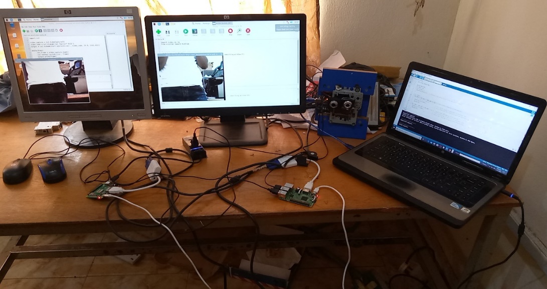
The system uses two Raspberry Pi computers (R-Pi 1 and R-Pi 2). R-Pi 1 runs the modified optical flow algorithm, written with Python and OpenCV. R-Pi 2 only records video, using a separate Python-OpenCV script. A vibration rig shakes the cameras so that the two outputs can be compared under the same conditions.

3.1Hardware

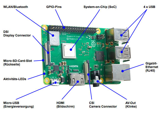
Each Raspberry Pi unit consists of a Raspberry Pi board (Figure 1), a camera, a power supply, an SD card and a display monitor. Because there are two units, each of these items is used in pairs. A Raspberry Pi model 3B+ was used, and a USB camera (Model V2) was connected to it. The vibration rig uses an Arduino UNO (Figure 2), an SG90 micro servo motor and a laptop computer.

3.2Stabilization algorithm

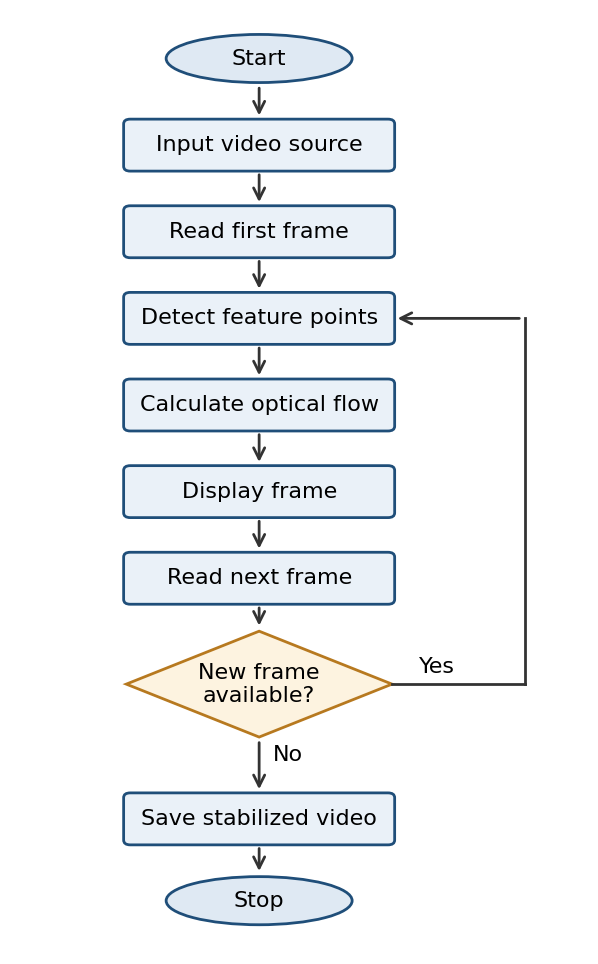
Raspbian, Python and OpenCV were installed on both boards. The modified optical flow algorithm was written on R-Pi 1, and the recording script on R-Pi 2. Figure 3 shows the flow of the algorithm. After reading the input video and its first frame, the program detects feature points and calculates their optical flow. It displays the frame, reads the next one and checks whether a new frame is available. If so, the loop returns to feature detection. If not, the stabilized video is saved and the program stops.

The optical flow algorithm was modified by adjusting the tracking features: the number of tracking features was reduced to 3, the window size was reduced to 30 so that the algorithm runs in real time, and the Lucas Haris feature detector was used.

3.3Vibration rig

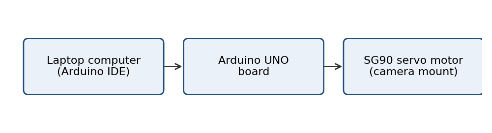
The rig is made of an Arduino UNO, an SG90 servo motor and a laptop (Figure 4). The laptop is connected to the Arduino board, which drives the servo motor. Vibration amplitude and frequency are set in the Arduino IDE on the laptop: the servo angle sets the amplitude, and the delay time in the program sets the frequency.

3.4Experimental setup

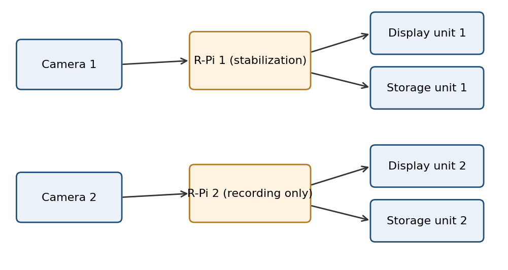
Each Raspberry Pi was connected to its own camera, storage and display (Figure 5). Both cameras were mounted on the vibration rig (Figure 6). Camera 1 fed R-Pi 1, which stabilized the video and sent it to display unit 1 and storage unit 1. Camera 2 fed R-Pi 2, which only displayed and stored the unprocessed, shaky video on display unit 2 and storage unit 2. Both cameras therefore saw the same vibration at the same time.

3.5Test procedure and evaluation

We recorded twelve videos from each Raspberry Pi with the two cameras on the rig, changing the vibration frequency for every recording. All videos were saved in AVI format at 640 × 480 pixels and 50 frames per second. For each frequency, the stabilized video from R-Pi 1 was compared with the shaky video from R-Pi 2 using the video quality measurement tool of Martínez-Rach et al. [22] and Vranjes [23]. We computed the average peak signal-to-noise ratio (PSNR) and the average video quality metric (VQM) for each pair.

PSNR is defined from the mean squared error (MSE) between two frames as PSNR = 10 log₁₀(255² / MSE), in dB for 8-bit images. A higher value indicates a steadier video [21]. For VQM, a lower score indicates better quality. The PSNR was computed between paired stabilized and shaky frames.

4Results and discussion

Figure 7 plots average PSNR against vibration frequency for the stabilized and shaky videos, and Table 1 lists the values. The stabilized video had the higher PSNR at eleven of the twelve frequencies. At 0.76 Hz the two were equal (22.1 dB).

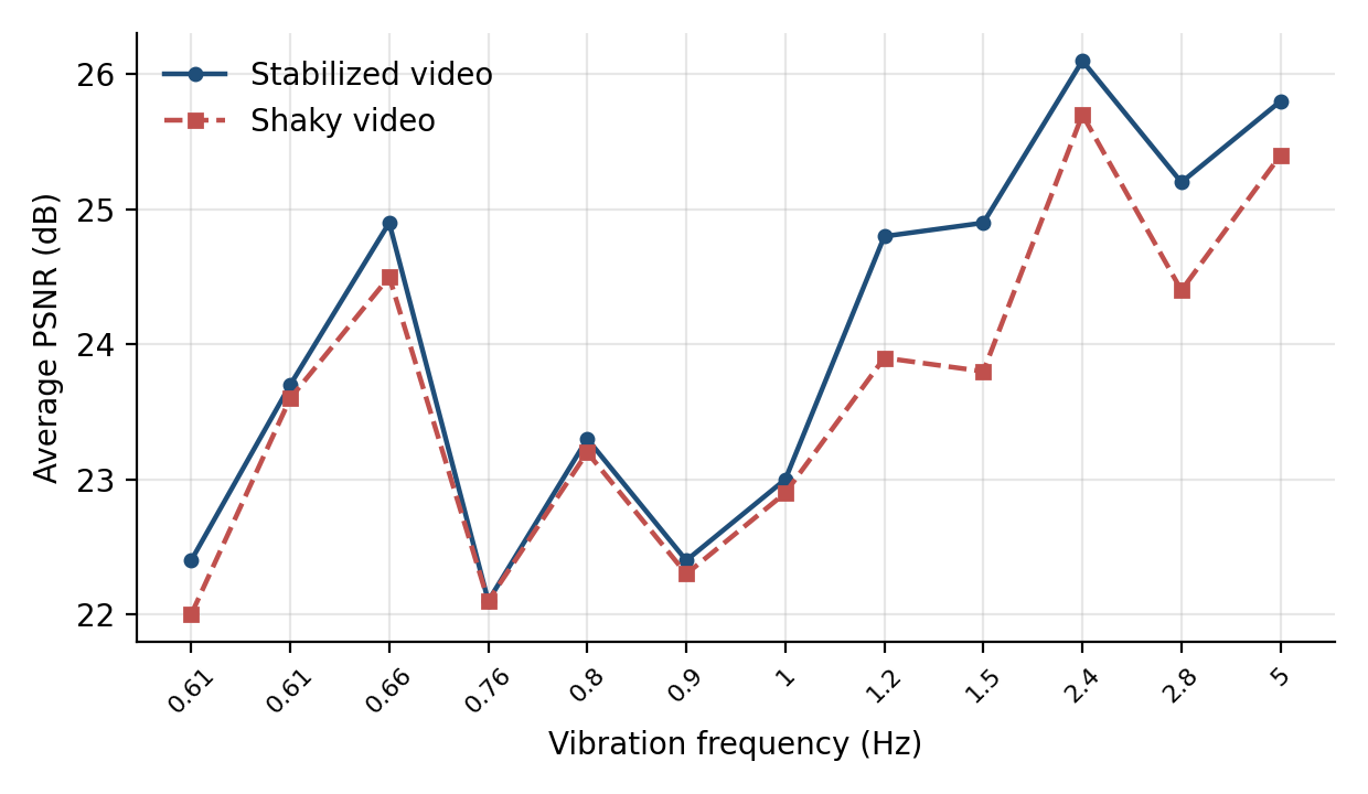
The gains are small in absolute terms. The mean is 0.4 dB across the twelve recordings, and the largest, 1.1 dB, occurs at 1.5 Hz, which is about 4.6% above the shaky video’s 23.8 dB. The frequency matters. Below 1.2 Hz the mean gain is 0.17 dB, while from 1.2 Hz upward it is 0.72 dB. In other words, the algorithm helps most when the shaking is faster. Two recordings were made at 0.61 Hz and gave different results (0.4 dB and 0.1 dB). The constraints of the vibration rig limited the range of frequencies that could be set.

Frequency (Hz)	Stabilized PSNR (dB)	Shaky PSNR (dB)	Gain (dB)
0.61	22.4	22.0	0.4
0.61	23.7	23.6	0.1
0.66	24.9	24.5	0.4
0.76	22.1	22.1	0.0
0.80	23.3	23.2	0.1
0.90	22.4	22.3	0.1
1.00	23.0	22.9	0.1
1.20	24.8	23.9	0.9
1.50	24.9	23.8	1.1
2.40	26.1	25.7	0.4
2.80	25.2	24.4	0.8
5.00	25.8	25.4	0.4

Two limits should be kept in mind. The two cameras sit side by side, so they do not see exactly the same view, and the results come from a bench rig at twelve frequencies. They are best read as preliminary.

The processing frame rate recorded on the Raspberry Pi 3B+ was 30 frames per second, and the frame delay was about 5 ms.

5Conclusion

We built a real-time video stabilizer on a Raspberry Pi using a modified optical flow algorithm and tested it on a vibration rig made from an Arduino UNO and a servo motor. Across twelve vibration frequencies, the stabilized video had an average PSNR at least as high as the shaky video, with a mean gain of 0.4 dB and a maximum of 1.1 dB at 1.5 Hz. The gain was larger above 1.2 Hz than below it, and at 0.76 Hz there was none. Authors: the original conclusion cites a 1.8% improvement at 0.61 Hz for PSNR.

Next steps are to report processing speed and latency on the board, to test on real moving platforms such as vehicles, and to compare the algorithm with other stabilizers on the same videos.

References

1. [1]Xu J, Chang HW, Yang S, Wang M. Fast feature-based video stabilization without accumulative global motion estimation. IEEE Transactions on Consumer Electronics. 2012;58(3):993–999.
2. [2]Rouhafzay A. Video stabilization using point feature matching. 2015.
3. [3]Windau J, Itti L. Multilayer real-time video image stabilization. In: 2011 IEEE/RSJ International Conference on Intelligent Robots and Systems. IEEE; 2011. p. 2397–2402.
4. [4]Karpenko A, Jacobs D, Baek J, Levoy M. Digital video stabilization and rolling shutter correction using gyroscopes. Stanford Computer Science Technical Report CSTR 2011-03. 2011.
5. [5]e Souza MR, Pedrini H. Visual rhythms for qualitative evaluation of video stabilization. EURASIP Journal on Image and Video Processing. 2020;2020(1):19.
6. [6]Ljubičić R, Strelnikova D, Perks MT, Eltner A, Peña-Haro S, Pizarro A, et al. A comparison of tools and techniques for stabilising UAS imagery for surface flow observations. Hydrology and Earth System Sciences Discussions. 2021;2021:1–42.
7. [7]Morimoto C, Chellappa R. Automatic digital image stabilization. In: Proceedings of the IEEE International Conference on Pattern Recognition; Vienna, Austria; 1996.
8. [8]Kornilova AV, Kirilenko IA, Zabelina NI. Real-time digital video stabilization using MEMS-sensors. Proceedings of the Institute for System Programming of the RAS. 2017;29(4):73–86.
9. [9]Bayrak S. Video stabilization: digital and mechanical approaches [Master’s thesis]. Ankara, Turkey: Middle East Technical University; 2008.
10. [10]Matsushita Y, Ofek E, Ge W, Tang X, Shum HY. Full-frame video stabilization with motion inpainting. IEEE Trans Pattern Anal Mach Intell. 2006;28(7):1150–1163.
11. [11]Liu F, Gleicher M, Jin H, Agarwala A. Content-preserving warps for 3D video stabilization. ACM Trans Graph. 2009;28(3).
12. [12]Zhang G, Hua W, Qin X, Shao Y, Bao H. Video stabilization based on a 3D perspective camera model. Vis Comput. 2009;25(11):997–1008.
13. [13]Grundmann M, Kwatra V, Essa I. Auto-directed video stabilization with robust L1 optimal camera paths. In: Proc. IEEE Conf. Comput. Vis. Pattern Recognit. (CVPR); 2011. p. 225–232.
14. [14]Goldstein A, Fattal R. Video stabilization using epipolar geometry. ACM Trans Graph. 2012;31(5).
15. [15]Liu S, Yuan L, Tan P, Sun J. Bundled camera paths for video stabilization. ACM Trans Graph. 2013;32(4).
16. [16]Liu S, Wang Y, Yuan L, Bu J, Tan P, Sun J. Video stabilization with a depth camera. In: 2012 IEEE Conference on Computer Vision and Pattern Recognition. IEEE; 2012. p. 89–95.
17. [17]Smith BM, Zhang L, Jin H, Agarwala A. Light field video stabilization. In: 2009 IEEE 12th International Conference on Computer Vision. IEEE; 2009. p. 341–348.
18. [18]Yu J, Ramamoorthi R. Selfie video stabilization. In: Proc. Eur. Conf. Comput. Vis. (ECCV); 2018.
19. [19]Yu J, Ramamoorthi R. Robust video stabilization by optimization in CNN weight space. In: Proc. IEEE/CVF Conf. Comput. Vis. Pattern Recognit. (CVPR); 2019. p. 3800–3808.
20. [20]Yu J, Ramamoorthi R. Learning video stabilization using optical flow. In: Proc. IEEE/CVF Conf. Comput. Vis. Pattern Recognit. (CVPR); 2020. p. 8159–8167.
21. [21]Deng Z, Yang D, Zhang X, Dong Y, Liu C, Shen Q. Real-time image stabilization method based on optical flow and binary point feature matching. Electronics. 2020;9(1):198.
22. [22]Martínez-Rach MO, Piñol P, López OM, Perez Malumbres M, Oliver J, Calafate CT. On the performance of video quality assessment metrics under different compression and packet loss scenarios. The Scientific World Journal. 2014;2014(1):743604.
23. [23]Vranjes I, Baillien E, Vandebosch H, Erreygers S, De Witte H. When workplace bullying goes online: Construction and validation of the Inventory of Cyberbullying Acts at Work (ICA-W). European Journal of Work and Organizational Psychology. 2018;27(1):28–39.