Micro-Catchment Typology for Integrated Catchment Management

1Introduction

Integrated catchment management seeks to coordinate land and water interventions across a drainage basin so that actions taken in one place do not create problems in another [1]. In practice, especially in data-scarce tropical regions, catchment assessments are often organised by hazard: an erosion map identifies areas for soil conservation, a flood map identifies areas for flood control, and a suitability map identifies sites for water harvesting. Each map produces its own priority list, and planners must reconcile them informally. The result is that interventions may be duplicated, may conflict, or may miss land units where several problems coincide.

Catchment classification offers an alternative. By grouping land units according to the similarity of their physical and hydrological characteristics, classification provides a basis for transferring understanding and management prescriptions among units that behave alike [2]. Multivariate methods such as principal component analysis (PCA) and cluster analysis are well suited to this task because they reduce correlated indicators to a few interpretable dimensions and group units objectively [3]. In watershed prioritisation, however, multivariate methods have mostly been used to reduce morphometric parameters before ranking [4], rather than to combine morphometric, erosional, hydrological and suitability information into management types. Classifications are also rarely tested for stability and spatial coherence, or used to estimate what zone-specific interventions would achieve, although both are needed before a typology can guide investment.

Catchments draining to the Niger–Benue confluence in north-central Nigeria illustrate the need for an integrated approach. Their dissected uplands generate rapid runoff and gully erosion, while their lowlands are cultivated and flood-prone; Kogi State is among the most flood-affected states in the country [5]. Interventions designed for one hazard can worsen another, for example where water-harvesting structures are placed on land that floods. This study therefore aimed to develop and evaluate a micro-catchment typology for integrated catchment management in such a setting. The objectives were to (i) assemble complementary indicators of geomorphic condition, erosion, runoff, flood exposure and harvesting potential for each micro-catchment; (ii) identify the main gradients of variation and group the micro-catchments into management zones; (iii) test the robustness and spatial coherence of the zones; (iv) characterise the zones by their hazard loads, groundwater recharge potential, population exposure, forest loss and rainfall trends; and (v) estimate the effect of zone-specific intervention and land-use scenarios on soil loss and runoff and rank priority units within each zone.

2Materials and methods

2.1Study area

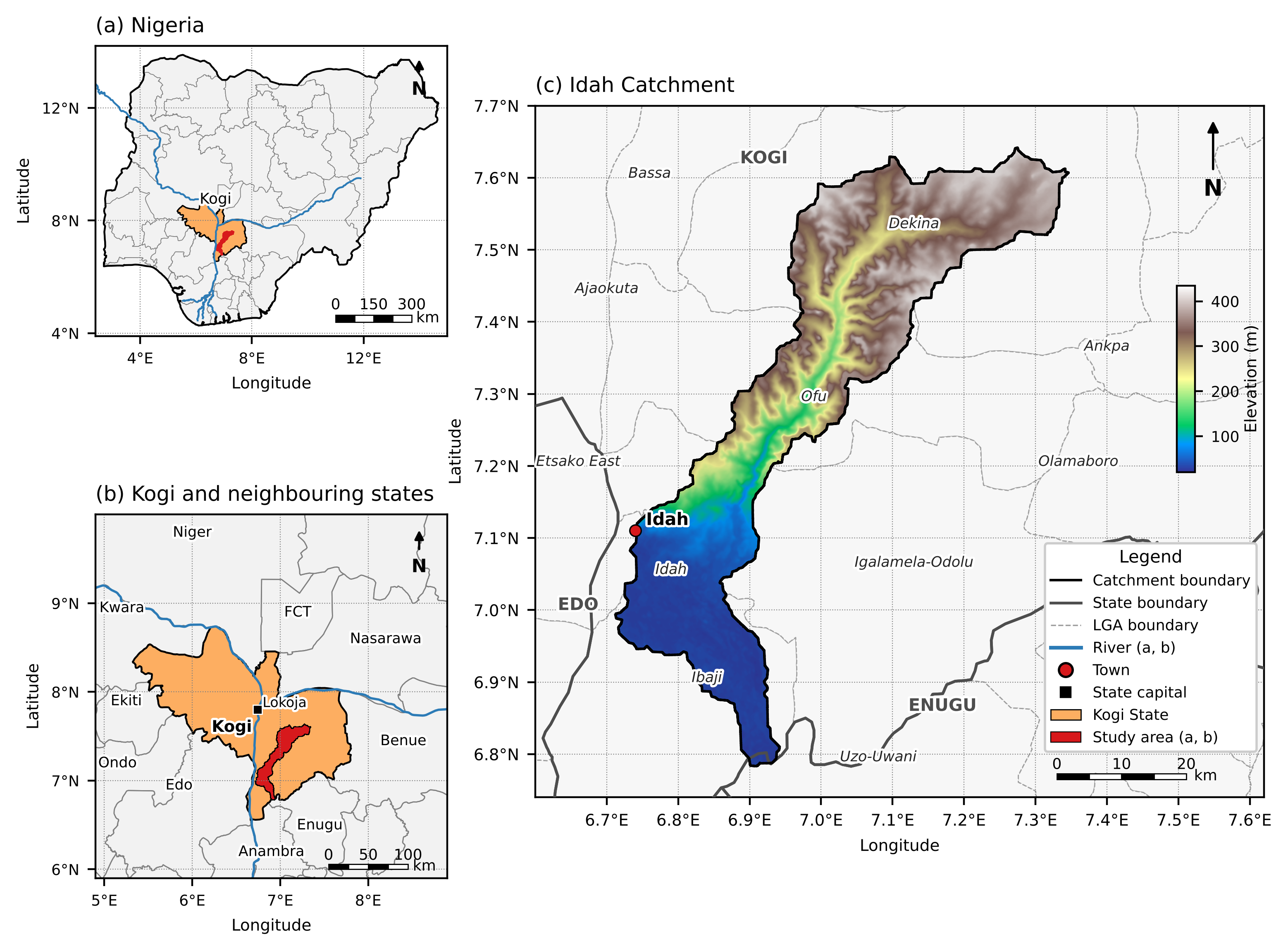
The Idah Catchment covers 1,641.7 km² in eastern Kogi State, Nigeria, between latitudes 6.78° and 7.64° N and longitudes 6.70° and 7.35° E (Figure 1). It lies almost entirely within Kogi State and spans five local government areas: Dekina (590 km²), Ofu (440 km²), Ibaji (301 km²), Igalamela-Odolu (248 km²) and Idah (58 km²). It drains south-westward from a wooded sandstone plateau at 434 m to the River Niger floodplain near Idah at 21 m. The catchment lies within the Cretaceous Anambra Basin, with Tertiary and Quaternary deposits towards the Niger [6, 7]. Land cover is dominated by tree cover (74.0%), with grassland (9.8%), shrubland (7.8%) and cropland (6.3%), the latter concentrated on the lowland [8].

2.2Micro-catchments and data

The 12.5 m ALOS PALSAR radiometrically terrain-corrected DEM [11] was geoid-corrected, projected to UTM zone 32N and hydrologically conditioned with a breach–fill algorithm [12]. The catchment was partitioned into micro-catchments with a 10 km² target area using the isobasin method, and the 163 complete units, covering 1,540.1 km² (93.8% of the catchment), formed the units of analysis. Rainfall was obtained from CHIRPS [13], soil texture from SoilGrids 2.0 [14] and land cover from ESA WorldCover 2021 [8]. Population in 2020 was taken from WorldPop at 100 m [15], built-up surface in 2020 from the Global Human Settlement Layer [16], and forest cover in 2000 and its loss in 2001–2023 from the Global Forest Change dataset version 1.11 [17]. These datasets were summarised for each micro-catchment in Google Earth Engine.

2.3Indicators

Nine indicators were selected to represent five dimensions of catchment condition: geomorphic form, erosion, runoff, flood exposure and water-harvesting potential (Table 1). The morphometric compound parameter was computed from ten linear, areal and relief parameters [4] and multiplied by −1 so that higher values denote higher priority. The hypsometric integral followed the elevation–relief ratio [18]. Mean annual soil loss was estimated with the Revised Universal Soil Loss Equation [19] and log-transformed to reduce skewness, and the mean cover-management factor (C) was retained as an indicator of land-use pressure. The curve number followed USDA-NRCS [20], and specific peak discharge was the 100-year SCS peak divided by unit area. Flood susceptibility and rainwater-harvesting (RWH) suitability were AHP-weighted indices [21], the former dominated by height above nearest drainage [22].

Dimension	Indicator	Unit	Median (range)
Geomorphic form	Morphometric priority (−Cp)	rank	−78.7 (−126.9 to −34.5)
Geomorphic form	Hypsometric integral (HI)	–	0.45 (0.10–0.66)
Geomorphic form	Mean slope	degrees	3.84 (1.56–7.33)
Erosion	Mean soil loss (RUSLE)	t ha−1 yr−1	2.71 (1.13–15.78)
Erosion / land use	Mean cover-management factor (C)	–	0.019 (0.010–0.185)
Runoff	Curve number (CN)	–	61.9 (55.1–80.5)
Runoff	Specific 100-year peak discharge	m3 s−1 km−2	1.70 (0.53–7.03)
Flood exposure	Flood susceptibility index	1–5	2.53 (1.91–4.26)
Harvesting potential	RWH suitability index	1–5	2.88 (2.06–4.48)

Note: Soil loss was log-transformed (ln(1 + A)) before analysis. All indicators were standardised to zero mean and unit variance.

2.4Principal component and cluster analysis

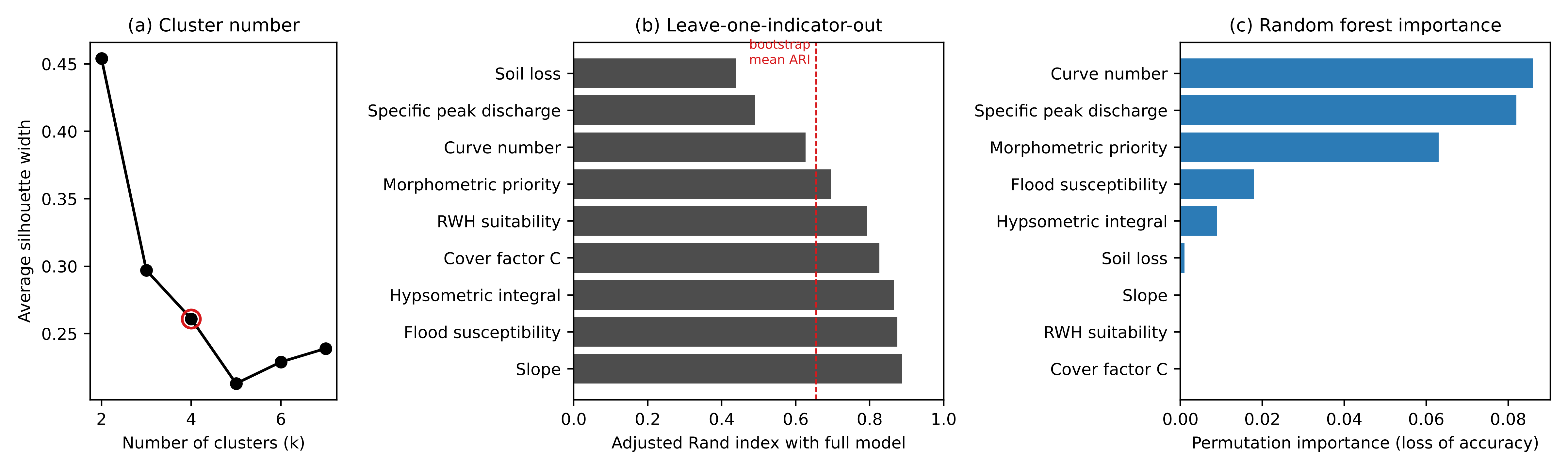
The standardised indicators were analysed with PCA to identify the main gradients of variation [3]. The units were then grouped with k-means clustering [23] on all nine standardised indicators, using 100 random initialisations. The number of clusters was chosen by combining the average silhouette width [24] for k = 2 to 7 with interpretability for management, since the solution with the highest silhouette may be too coarse to guide interventions. Differences in indicators among zones were tested with the Kruskal–Wallis test.

Robustness was assessed in four ways, using the adjusted Rand index (ARI) [25] to compare partitions. First, the k-means partition was compared with Ward's hierarchical clustering [26]. Second, k-means was re-fitted to 200 bootstrap samples and the predicted partitions compared with the original [27]. Third, each indicator was removed in turn and the clustering repeated, to identify indicators on which the zones depend. Fourth, a random forest of 1,000 trees [28] was trained to predict the zones from the indicators; its out-of-bag accuracy measured how well the zones are separable, and permutation importance (50 repeats) measured each indicator's contribution.

2.5Spatial coherence

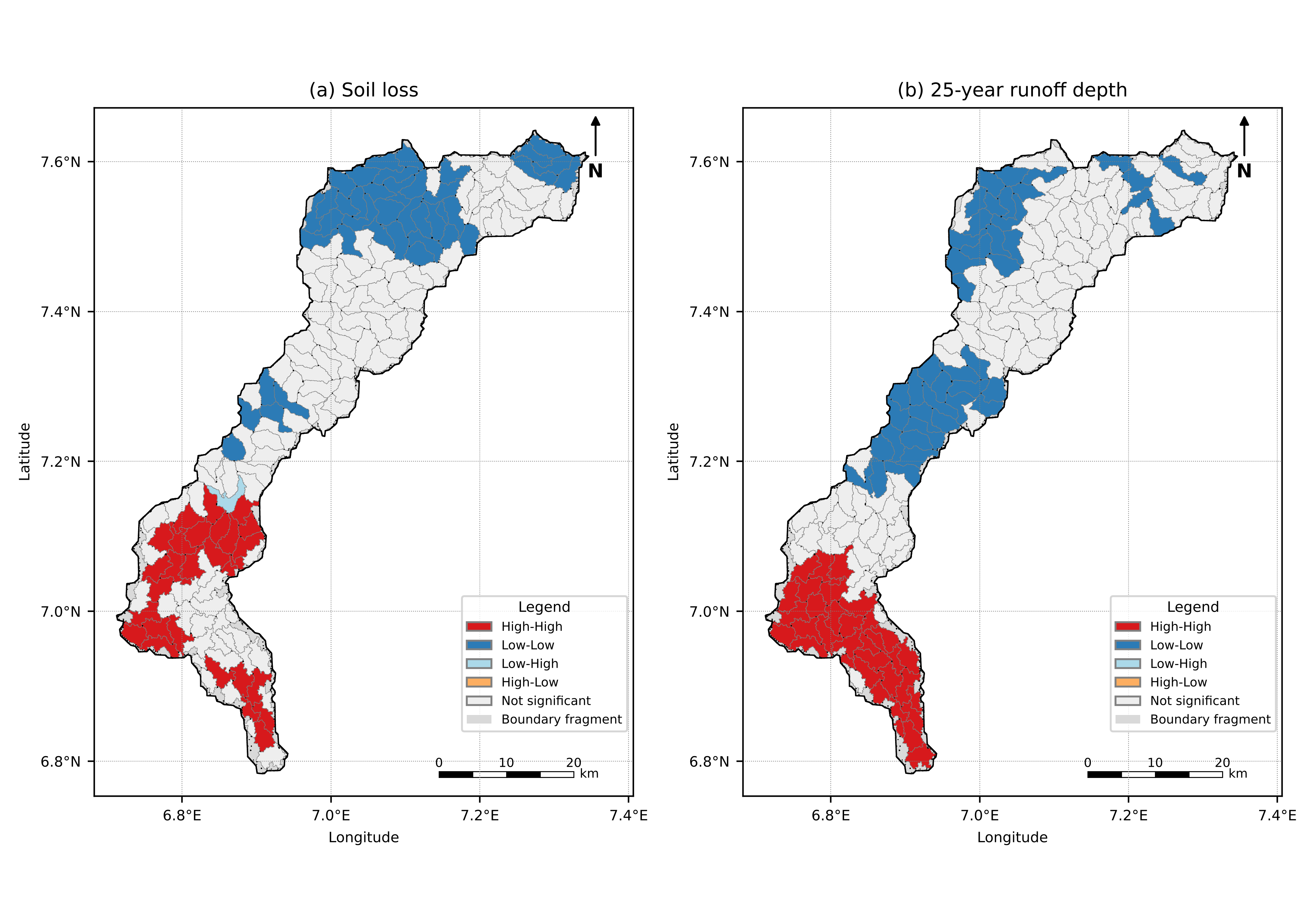
Because the clustering ignored location, the spatial arrangement of the zones provides an independent check on their physical meaning. Spatial weights were defined by queen contiguity between micro-catchment polygons and row-standardised. Global Moran's I [29] was computed for each indicator, and the share of neighbouring pairs belonging to the same zone was compared with its distribution under 999 random relabellings of the zones. Local indicators of spatial association (LISA) [30] were computed for mean soil loss and 25-year runoff depth to locate significant high–high hotspots and low–low coldspots (999 permutations, p < 0.05). The analyses used PySAL [31].

2.6Zone loads, recharge potential, exposure and rainfall trends

For each zone, total soil loss (t yr⁻¹) and total 25-year runoff volume (m³) were summed and expressed as shares of the totals for the 163 units. Groundwater recharge potential was mapped with a revised AHP overlay in which geology was added (Cretaceous = 3, Quaternary = 4, Tertiary = 5) and lineament density was given the lowest importance, because in the original model its quantile scores collapsed into two classes and dominated the highest-potential class. The resulting weights were geology 33.1%, slope 23.1%, rainfall 15.7%, drainage density 10.6%, soil 7.1%, land cover 4.8%, topographic wetness 3.3% and lineament density 2.4% (consistency ratio 0.029). For each unit, the mean index and the share of the unit in the top 20% of the catchment's index values were extracted. Population, built-up surface, forest cover in 2000 (tree cover of at least 30%) and forest loss in 2001–2023 were summed for each zone. Annual rainfall and annual maximum daily rainfall from CHIRPS for 1995–2024 were averaged over each zone, weighted by unit area, and tested for monotonic trend with the Mann–Kendall test [32, 33], with the trend magnitude given by Sen's slope [34].

2.7Intervention and land-use scenarios

Four soil-loss scenarios were applied to the RUSLE rasters at 12.5 m. In S1, the cover-management factor of cropland pixels in Zone 3 was reduced from 0.25 to 0.10 to represent conservation agriculture with cover crops, mulching and minimum tillage [35]. In S2, contour bunds were added on the same cropland, with the support-practice factor P set by slope class from 0.5 to 1.0 [36]; P was 1 in the baseline. S3 extended S2 to cropland in Zone 4. S4 was a degradation scenario in which 20% of the tree cover in Zone 1 was converted to cropland; it was implemented as the expected value over all tree pixels, multiplying soil loss by 1 + 0.2 (0.25/C − 1), where C is the existing cover factor.

Four runoff scenarios were evaluated for the 25-year, 24-hour design storm with the SCS curve-number method [20], using each unit's design rainfall and an initial abstraction ratio of 0.2. In R1 and R2, the curve number of each unit in Zone 3, and in Zones 3 and 4, respectively, was reduced by six units multiplied by the unit's cropland fraction, representing improved infiltration under conservation agriculture. In R3, the first-fill storage of 126 candidate check dams in Zones 1 to 3 from a previous siting analysis was subtracted from the runoff of the unit in which each dam lies, without exceeding that runoff; dams in Zone 4 and dams whose pond reached the edge of the search window were excluded. R4 combined R2 and R3.

2.8Within-Zone prioritisation and intervention packages

Units within each zone were ranked by a zone-specific score, the mean of min–max normalised indicators chosen to match the zone's management objective: morphometric priority, HI and specific peak discharge in Zone 1 (headwater protection); specific peak discharge, slope and morphometric priority in Zone 2 (peak attenuation); soil loss, specific peak discharge and cover factor in Zone 3 (source control); and flood susceptibility, curve number and soil loss in Zone 4 (flood-risk reduction). Intervention packages were then assigned to each zone from its indicator profile and the scenario results, following established soil and water conservation and flood-management practice.

3Results

3.1Main gradients of variation

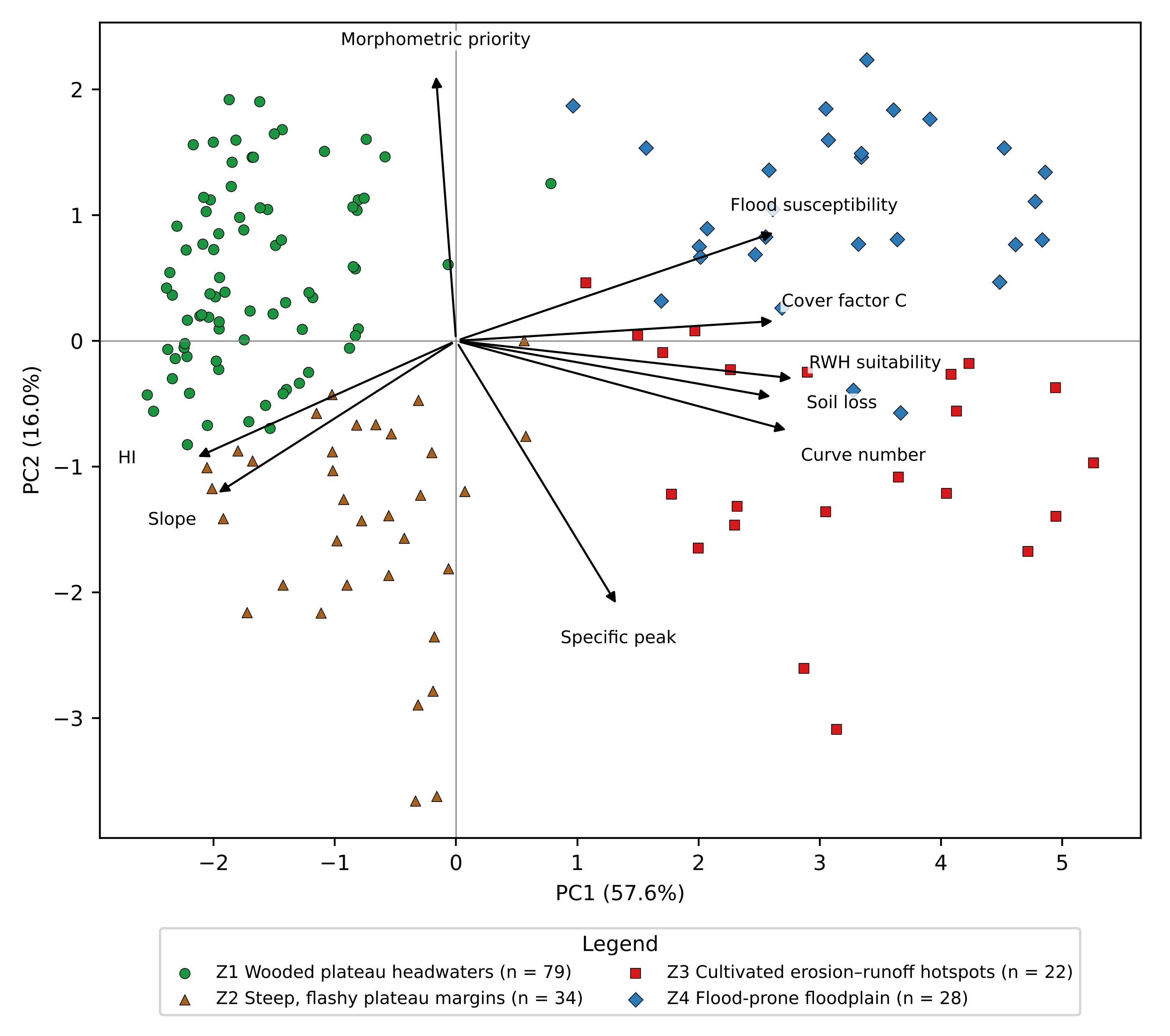
The first two principal components explained 57.6% and 16.0% of the variance (73.6% together), and the first four components explained 90.0% (Table 2; Figure 2). PC1 had strong positive loadings for RWH suitability (0.94), curve number (0.92), soil loss, flood susceptibility and cover factor (0.88 each), and negative loadings for HI (−0.72) and slope (−0.66). It therefore represents a gradient from wooded, steep, high-integral plateau units to cultivated, runoff-generating, flood-prone lowland units. PC2 contrasted morphometric priority (0.71) with specific peak discharge (−0.71), separating elongated, densely drained units from compact units that produce high peaks per unit area.

Indicator	PC1	PC2	PC3
Morphometric priority	−0.06	0.71	0.69
Hypsometric integral	−0.72	−0.31	0.24
Mean slope	−0.66	−0.41	0.02
Soil loss	0.88	−0.15	0.02
Curve number	0.92	−0.24	0.10
Specific peak discharge	0.45	−0.71	0.47
Flood susceptibility	0.88	0.29	−0.13
RWH suitability	0.94	−0.10	0.04
Cover-management factor	0.88	0.05	−0.02
Variance explained (%)	57.6	16.0	8.7

Note: Loadings are correlations between the standardised indicators and the components.

3.2Management Zones

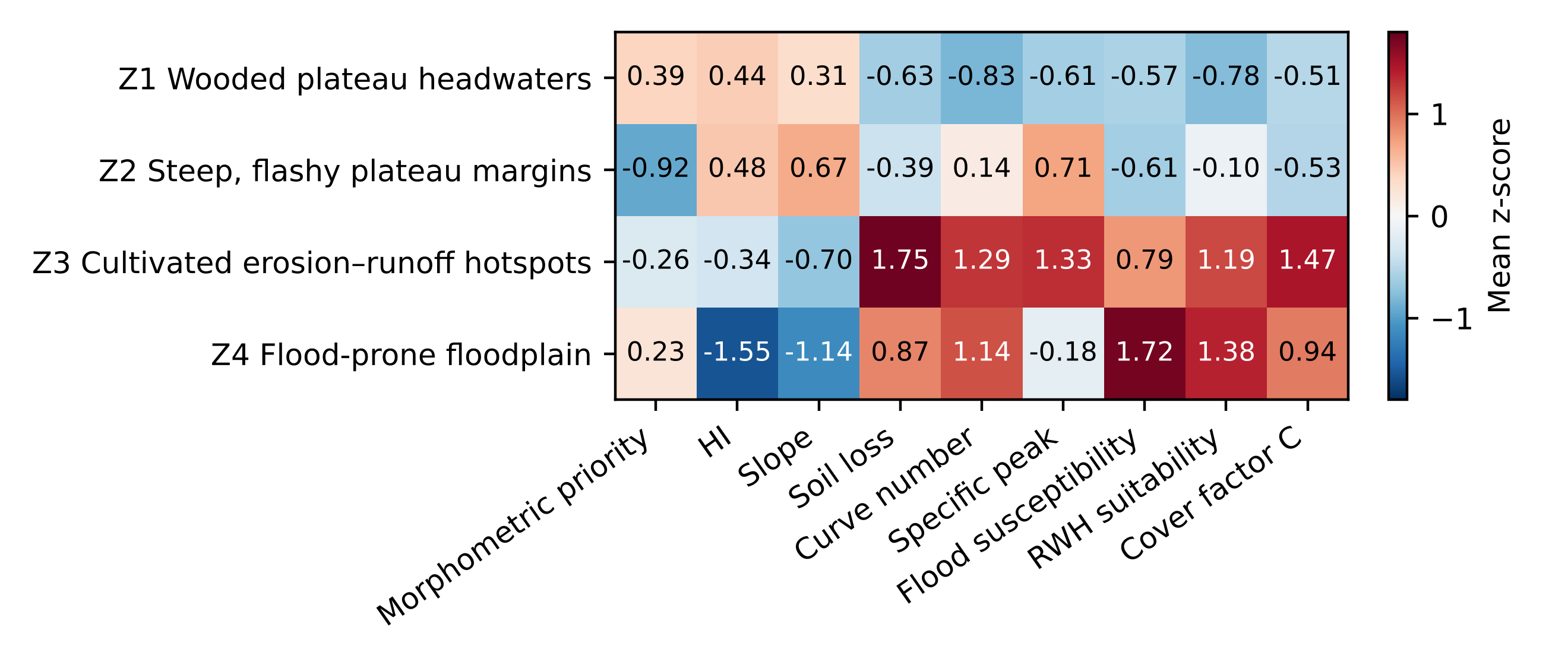
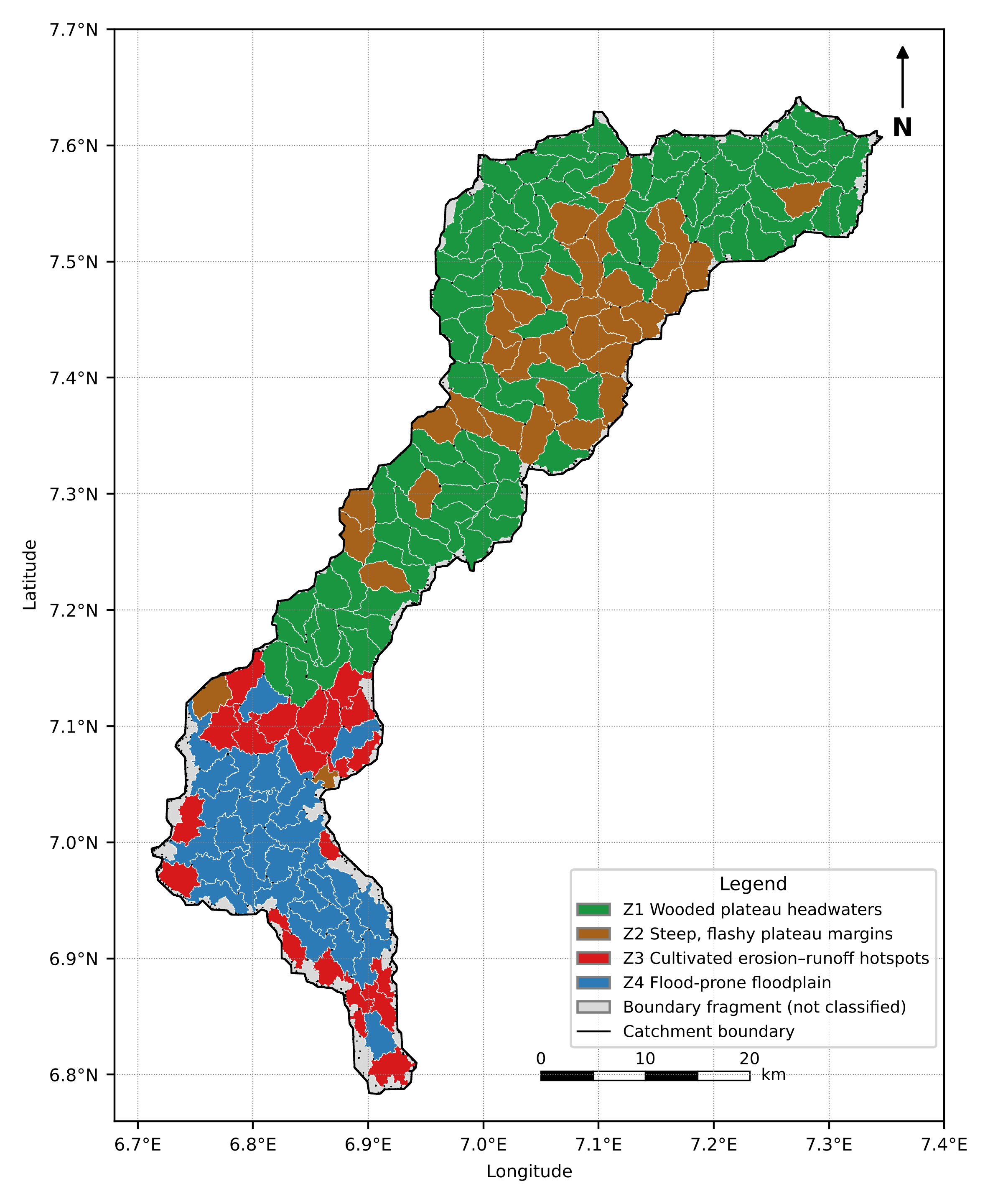
The average silhouette width was highest for two clusters (0.45) and was 0.26 for four clusters. The two-cluster solution simply separated upland from lowland, so the four-cluster solution was retained because it distinguished management-relevant contrasts within each. All nine indicators differed significantly among zones (Kruskal–Wallis p < 10⁻⁸). The zone profiles are shown in Figure 3 and Table 3, and their distribution in Figure 4.

Variable	Z1 Wooded plateau headwaters	Z2 Steep, flashy plateau margins	Z3 Cultivated erosion–runoff hotspots	Z4 Flood-prone floodplain
Micro-catchments (n)	79	34	22	28
Area (km2; % of analysed area)	770.9 (50.1)	334.6 (21.7)	160.8 (10.4)	273.9 (17.8)
Mean elevation (m)	318	316	41	32
Compound parameter Cp	72.6	99.1	87.8	73.0
Hypsometric integral	0.49	0.50	0.37	0.22
Mean slope (°)	4.3	4.8	3.2	2.9
Soil loss (t ha−1 yr−1)	2.0	2.5	8.4	5.6
Area with soil loss > 20 t ha−1 yr−1 (%)	0.6	0.7	10.9	7.7
Cover-management factor C	0.016	0.015	0.066	0.071
Curve number	56.8	65.7	73.9	74.3
Specific qp100 (m3 s−1 km−2)	1.23	2.94	3.52	1.81
100-year runoff depth (mm)	6.4	13.3	23.4	25.7
Flood susceptibility index	2.42	2.38	3.19	3.84
RWH suitability index	2.56	3.02	4.05	4.27
High-priority units by Cp (n)	36	2	4	12
Candidate check dams (n; storage Mm3)	49 (1.45)	56 (0.95)	30 (1.54)	15 (0.86)

Note: Lower Cp denotes higher morphometric priority.

Zone 1, wooded plateau headwaters (79 units, 50.1% of the analysed area), combined the lowest curve number (56.8), lowest specific peak discharge (1.23 m³ s⁻¹ km⁻²), low soil loss (2.0 t ha⁻¹ yr⁻¹) and extensive tree cover (88.0% of its area in the WorldCover tree-cover class; C = 0.016) with high HI (0.49). It nevertheless contained 36 of the 54 morphometrically high-priority units, which are elongated and densely drained.

Zone 2, steep, flashy plateau margins (34 units, 21.7%), was also wooded and had low soil loss, but it had the steepest slopes (4.8°), a higher curve number (65.7) and specific peak discharges more than twice those of Zone 1 (2.94 m³ s⁻¹ km⁻²). Most of its units were of low morphometric priority (25 of 34).

Zone 3, cultivated erosion–runoff hotspots (22 units, 10.4%), lay on the lowland margins (median elevation 41 m) and had the highest soil loss (8.4 t ha⁻¹ yr⁻¹), the largest share of land losing more than 20 t ha⁻¹ yr⁻¹ (10.9%), the highest specific peak discharge (3.52 m³ s⁻¹ km⁻²) and a high cover factor (0.066), reflecting cultivation.

Zone 4, flood-prone floodplain (28 units, 17.8%), had the lowest HI (0.22) and slope (2.9°), the highest curve number (74.3), runoff depth (25.7 mm at T = 100 years), flood susceptibility (3.84) and RWH suitability (4.27), and the highest cover factor (0.071).

3.3Robustness and spatial coherence of the Zones

The four-zone partition was moderately stable (Table 4). It agreed with Ward's clustering (ARI = 0.69), and bootstrap re-fitting gave a mean ARI of 0.655 (5th–95th percentile 0.44–0.87). The random forest reproduced the zones with an out-of-bag accuracy of 92.0%, showing that the zones are well separated in indicator space despite the modest silhouette width. Removing slope, flood susceptibility, HI or cover factor left the partition largely unchanged (ARI 0.83–0.89), whereas removing soil loss (ARI 0.44) or specific peak discharge (0.49) altered it substantially (Figure 5). In the random forest, curve number, specific peak discharge and morphometric priority were the most important indicators. Soil loss had low permutation importance even though the partition depended on it, because its information is largely duplicated by curve number and the cover factor.

Test	Statistic	Value
Agreement with Ward clustering	ARI	0.692
Bootstrap stability (200 resamples)	Mean ARI (5th–95th percentile)	0.655 (0.440–0.874)
Leave-one-indicator-out	ARI range	0.439 (soil loss) to 0.888 (slope)
Random forest (1,000 trees)	Out-of-bag accuracy	0.920
Global Moran's I, eight indicators	Range (p)	0.28–0.90 (0.001)
Global Moran's I, morphometric priority	I (p)	0.06 (0.106)
Same-zone neighbours	Observed vs random share (p)	0.653 vs 0.321 (0.001)
Soil-loss LISA	High–high / low–low units	28 / 39
Runoff-depth LISA	High–high / low–low units	32 / 43

Note: ARI = adjusted Rand index; LISA = local indicator of spatial association (999 permutations, p < 0.05).

Although location was not used in the clustering, the zones were strongly clustered in space. Eight of the nine indicators showed significant positive spatial autocorrelation (Moran's I 0.28–0.90, p = 0.001), the exception being morphometric priority (I = 0.06, p = 0.106), which varies from unit to unit. Neighbouring units belonged to the same zone in 65.3% of cases, twice the 32.1% expected by chance (p = 0.001). The LISA maps (Figure 6) placed the soil-loss hotspots almost entirely in the lowland: 12 of the 28 high–high units were in Zone 3 and 14 in Zone 4, while 30 of the 39 low–low units were in Zone 1. Runoff-depth hotspots were concentrated in the floodplain (23 of 32 high–high units in Zone 4 and 9 in Zone 3), and all 43 coldspots lay on the plateau (38 in Zone 1 and 5 in Zone 2).

3.4Contribution of Zones to Catchment loads

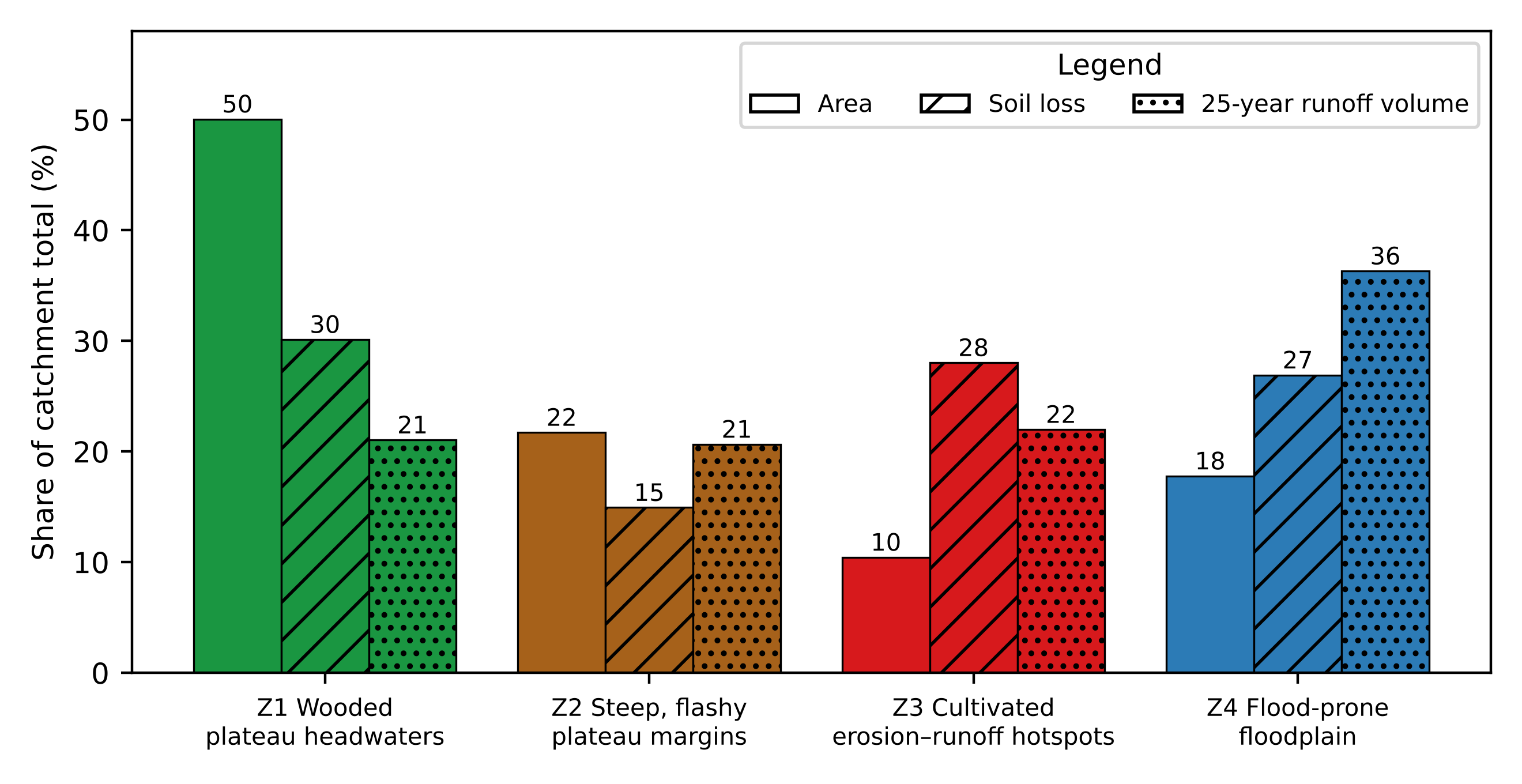
The zones contributed very unequally to catchment soil loss and runoff (Figure 7). Zone 1 occupied half of the analysed area but produced 30.1% of the soil loss (578,192 t yr⁻¹ in total) and 21.0% of the 25-year runoff volume (13.93 Mm³ in total). Zone 2 produced 14.9% of the soil loss and 20.7% of the runoff from 21.7% of the area. In contrast, Zone 3 produced 28.0% of the soil loss and 22.0% of the runoff from only 10.4% of the area, and Zone 4 produced 26.9% of the soil loss and 36.3% of the runoff from 17.8%. Together, Zones 3 and 4 occupied 28.2% of the analysed area but generated 54.9% of the soil loss and 58.3% of the runoff.

3.5Recharge potential, exposure, forest loss and rainfall trends

The zones also differed in groundwater recharge potential, population, forest loss and rainfall trends (Table 5). Recharge potential was highest in the lowland zones (Kruskal–Wallis p < 10⁻⁷): a median of 65.8% of each Zone 4 unit and 40.2% of each Zone 3 unit fell in the top 20% of the recharge index, compared with 2.8% and 2.0% in Zones 1 and 2. The 163 units held about 284,100 people in 2020. Most lived on the plateau: Zone 1 held 42.5% of the population and Zone 2 33.7%, and Zone 2 had the highest density (286 persons km⁻²) and the largest built-up surface (11.5 km²). Zone 4, the most flood-prone zone, held 12.3% of the population at 127 persons km⁻².

Variable	Z1	Z2	Z3	Z4
Median recharge index (1–5)	3.16	3.19	3.58	3.73
Median share of unit in top 20% of recharge index (%)	2.8	2.0	40.2	65.8
Population, 2020 (persons; % of total)	120,708 (42.5)	95,835 (33.7)	32,777 (11.5)	34,820 (12.3)
Population density (persons km−2)	157	286	204	127
Built-up surface, 2020 (km2)	6.63	11.48	2.11	1.29
Forest in 2000, ≥ 30% tree cover (km2)	38.7	23.4	1.1	10.3
Forest loss, 2001–2023 (km2; % of 2000 forest)	6.60 (17.0)	5.85 (25.0)	0.33 (30.2)	0.85 (8.3)
Mean annual rainfall, 1995–2024 (mm)	1,339	1,336	1,402	1,469
Sen's slope, annual rainfall (mm yr−1; p)	−2.70 (0.354)	−1.95 (0.432)	−8.48 (0.012)	−10.32 (0.006)
Mean annual maximum daily rainfall (mm)	45.2	45.0	48.2	50.0
Sen's slope, annual maximum (mm yr−1; p)	+0.24 (0.059)	+0.38 (0.030)	+0.07 (0.521)	0.00 (0.943)

Note: p values are from the Mann–Kendall test. Population from WorldPop, built-up surface from GHSL and forest from the Global Forest Change dataset (version 1.11).

Forest with at least 30% tree cover in 2000 covered only 73.5 km² (4.8% of the analysed area), much less than the WorldCover tree-cover class, which includes open woodland with tree cover of at least 10% and occupied 88.0% of Zone 1 and 82.9% of Zone 2. Closed forest therefore made up only 5.0% of Zone 1 and 7.0% of Zone 2, and the plateau is better described as woodland than as forest. Of this forest, 13.6 km² (18.5%) was lost between 2001 and 2023, mostly on the plateau (6.6 km² in Zone 1 and 5.9 km² in Zone 2), where the proportional loss was 17.0% and 25.0%. Annual rainfall declined significantly in the lowland zones, by 8.5 mm yr⁻¹ in Zone 3 (p = 0.012) and 10.3 mm yr⁻¹ in Zone 4 (p = 0.006), but showed no significant trend on the plateau. Annual maximum daily rainfall increased significantly only in Zone 2 (0.38 mm yr⁻¹, p = 0.030), with a weaker increase in Zone 1 (p = 0.059).

3.6Intervention and land-use scenarios

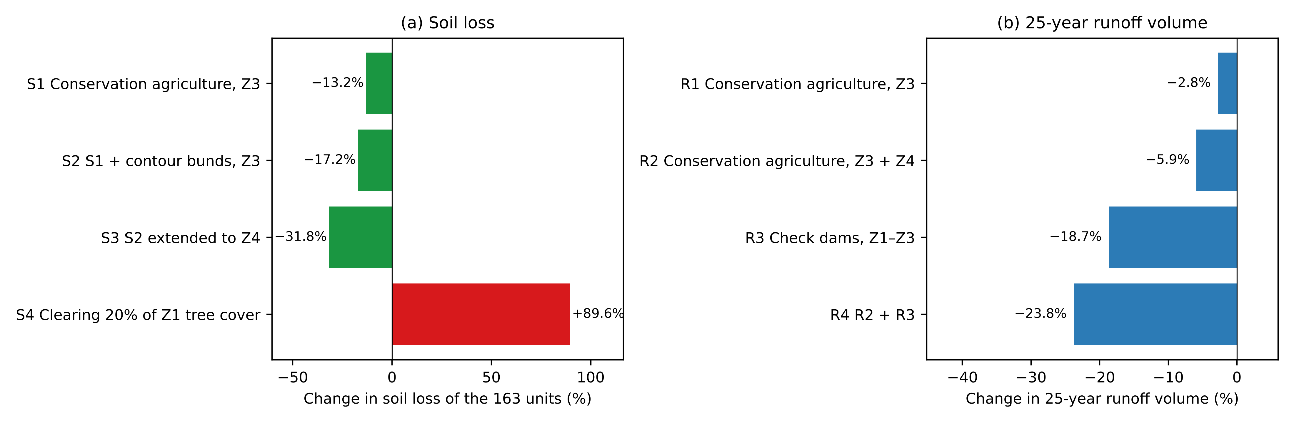
The scenarios showed that targeting the lowland cropland would reduce catchment loads substantially, while clearing headwater tree cover would more than offset these gains (Table 6; Figure 8). Conservation agriculture on Zone 3 cropland (S1) reduced soil loss in Zone 3 by 47.1% and in the 163 units by 13.2%. Adding contour bunds (S2) raised these reductions to 61.4% and 17.2%, and extending the package to Zone 4 cropland (S3) reduced Zone 4 soil loss by 54.3% and total soil loss by 31.8%, from 578,192 to 394,102 t yr⁻¹. In contrast, converting 20% of Zone 1 tree cover to cropland (S4) increased soil loss in Zone 1 almost fourfold (+297.3%) and total soil loss by 89.6%.

Curve-number reductions had smaller effects on runoff, because cropland is a small fraction of most units: the 25-year runoff volume fell by 12.7% in Zone 3 under R1 and by 8.5% in Zone 4 under R2, or 2.8% and 5.9% of the total. The first-fill storage of the 126 check dams in Zones 1 to 3 (R3) retained 2.61 Mm³, or 18.7% of the 25-year runoff, with reductions of 20.2% in Zone 1, 31.3% in Zone 2 and 36.3% in Zone 3. This assumes empty ponds; if the ponds were half full or three-quarters full at the start of the storm, retention would fall to 11.5% and 6.2% of the runoff. Combining conservation agriculture and check dams (R4) reduced the 25-year runoff volume by 23.8%, from 13.93 to 10.62 Mm³, and by 45.5% in Zone 3.

Scenario	Z1	Z2	Z3	Z4	All units
Soil loss (baseline, t yr−1)	174,186	86,359	162,067	155,581	578,192
S1 Conservation agriculture, Z3	0.0	0.0	−47.1	0.0	−13.2
S2 S1 + contour bunds, Z3	0.0	0.0	−61.4	0.0	−17.2
S3 S2 extended to Z4	0.0	0.0	−61.4	−54.3	−31.8
S4 Clearing 20% of Z1 tree cover	+297.3	0.0	0.0	0.0	+89.6
25-year runoff (baseline, Mm3)	2.93	2.88	3.06	5.06	13.93
R1 Conservation agriculture, Z3	0.0	0.0	−12.7	0.0	−2.8
R2 Conservation agriculture, Z3 and Z4	0.0	0.0	−12.7	−8.5	−5.9
R3 Check dams, Z1–Z3 (first fill)	−20.2	−31.3	−36.3	0.0	−18.7
R4 R2 + R3	−20.2	−31.3	−45.5	−8.5	−23.8

Note: Conservation agriculture: cropland C reduced from 0.25 to 0.10 and curve number reduced by up to six units; contour bunds: P by slope class (0.5–1.0). Check-dam storage assumes empty ponds at the start of the storm; with half-full ponds, R3 would be −11.5%.

3.7Priority units within Zones

The five highest-ranked units in each zone are listed in Table 7. In Zone 1, the top units combined high morphometric priority or high HI with specific peaks above the zone median (2.2–3.0 m³ s⁻¹ km⁻² in four of the five). The Zone 2 priorities had specific peaks of 3.6–5.3 m³ s⁻¹ km⁻². The Zone 3 priorities had soil loss of 12.6–15.8 t ha⁻¹ yr⁻¹, about 1.5 to 1.9 times the zone median, and curve numbers of 75–81, while the Zone 4 priorities had flood-susceptibility indices of 3.90–4.26.

Zone	Rank	Unit	Area (km2)	Soil loss (t ha−1 yr−1)	CN	qp100 (m3 s−1 km−2)	Flood index	Score
Z1	1	MC01687	6.9	1.7	60.7	2.57	2.20	0.755
Z1	2	MC01818	11.4	2.6	60.7	2.95	2.45	0.744
Z1	3	MC01804	10.0	1.8	63.8	2.64	2.57	0.729
Z1	4	MC01688	10.1	2.2	61.8	2.18	2.48	0.696
Z1	5	MC01800	9.4	1.9	56.0	1.09	2.33	0.684
Z2	1	MC01812	9.9	3.4	62.3	3.55	2.59	0.758
Z2	2	MC01169	12.4	3.3	60.7	3.65	2.31	0.709
Z2	3	MC01166	10.4	3.6	68.1	5.34	2.27	0.693
Z2	4	MC01802	10.6	2.3	65.3	4.27	2.45	0.678
Z2	5	MC01819	9.9	3.3	61.6	3.83	2.74	0.651
Z3	1	MC00697	9.0	15.8	75.4	3.01	2.74	0.731
Z3	2	MC00770	10.4	13.0	80.5	4.29	3.23	0.722
Z3	3	MC00786	10.1	13.2	78.8	4.24	3.53	0.715
Z3	4	MC00407	8.9	14.5	80.0	3.29	3.63	0.664
Z3	5	MC00634	9.5	12.6	78.5	4.01	3.95	0.641
Z4	1	MC00436	9.1	11.1	78.2	2.18	3.90	0.895
Z4	2	MC00473	10.0	9.6	78.2	1.70	3.92	0.863
Z4	3	MC00633	9.5	5.1	77.8	2.64	4.26	0.795
Z4	4	MC00632	9.4	6.2	77.4	2.45	4.04	0.770
Z4	5	MC00498	8.7	6.0	76.2	1.90	4.06	0.745

Note: The score is the mean of min–max normalised zone-specific indicators (Section 2.8) and is comparable only within a zone.

3.8Intervention packages

The intervention packages derived from the zone profiles and scenario results are summarised in Table 8. They differ in their primary objective: protection in Zone 1, peak attenuation in Zone 2, source control of erosion and runoff in Zone 3, and flood-risk reduction with flood-tolerant water storage and groundwater recharge in Zone 4.

Zone	Primary objective	Recommended interventions	Interventions to avoid
Z1 Wooded plateau headwaters	Protect tree cover and headwater function	Woodland and forest protection and community forestry, with priority to units losing forest; gully-head control in densely drained, high-priority units; small check dams on first-order channels; regulation of land clearing	Large-scale clearing for cultivation; road construction without drainage control
Z2 Steep, flashy plateau margins	Attenuate peak flows and prevent gullying	Check dams and gabion structures on low-order channels; riparian buffers; adequately sized culverts and drainage in built-up areas; enrichment planting on steep slopes	Cultivation on steep slopes; undersized crossings; unplanned urban expansion
Z3 Cultivated erosion–runoff hotspots	Control erosion and runoff at source	Conservation agriculture (cover crops, mulching, minimum tillage); contour bunds and vegetative strips; farm ponds and check dams to store runoff; agroforestry	Bare fallows during the wet season; down-slope tillage
Z4 Flood-prone floodplain	Reduce flood risk and use floodwater productively	Floodplain zoning and early warning; conservation agriculture with contour bunds on cropland; retention basins, raised farm ponds and managed aquifer recharge; flood-tolerant cropping; riparian vegetation	In-channel check dams; settlement and infrastructure in high-susceptibility areas

4Discussion

4.1A single dominant gradient

The dominance of PC1 shows that most hazard and opportunity indicators in this catchment vary together along an upland–lowland gradient. Curve number, cover factor, soil loss, flood susceptibility and RWH suitability all increase from the wooded plateau to the cultivated lowland. This co-variation explains why hazard-by-hazard maps in such catchments tend to highlight the same lowland areas, and it underlines the risk of conflicting recommendations: the lowland is simultaneously the most suitable for harvesting and the most flood-prone. Managing these interactions requires treating the lowland as a single management unit with its own combined objectives, which the typology achieves.

4.2Information beyond the main gradient

The second component and the four-zone solution reveal contrasts that a single upland–lowland division would hide. On the plateau, Zone 2 is distinguished from Zone 1 not by erosion but by its flashy hydrological response; its units have low morphometric priority yet produce the highest specific peaks outside the lowland. On the lowland, Zone 3 is distinguished from Zone 4 by erosion and peak runoff rather than flood exposure. The leave-one-out and random forest results confirm that these distinctions rest mainly on runoff and erosion indicators, while slope and flood susceptibility add little once the others are known. The weak and spatially random pattern of morphometric priority (Moran's I = 0.06) also indicates that morphometric ranking alone would scatter effort across the catchment, since most morphometrically high-priority units lie in the low-hazard Zone 1.

4.3Robustness and spatial meaning

The modest silhouette width (0.26) shows that the zones are not sharply separated clusters but segments of a continuum. This is expected for catchment properties that change gradually with relief and land use, and it does not prevent the zones from being useful: the random forest separated them with 92% accuracy, and their agreement with Ward clustering and bootstrap re-fits was moderate to good. The strong spatial coherence is more persuasive evidence of physical meaning. Clustering without coordinates produced contiguous zones, and the independently computed LISA hotspots of soil loss and runoff coincided with Zones 3 and 4. Units at zone boundaries and those whose assignment changes between re-fits should still be checked in the field before investment.

4.4What targeted interventions could achieve

The scenarios convert the zone loads into expected management gains. Because Zones 3 and 4 generate more than half of the soil loss from 28.2% of the area, applying conservation agriculture and contour bunds to their cropland would remove almost a third of the catchment's soil loss, a substantial effect from a measure applied only to the cropland within these two zones. The asymmetry with the degradation scenario is equally important. Clearing one-fifth of the headwater tree cover would add more soil loss than the lowland package removes, so protection of Zone 1 is not optional but a condition for lowland gains to persist. The forest-loss data suggest that this pressure is already real, with 17% of Zone 1 forest and 25% of Zone 2 forest lost since 2000, concentrated in the most populated part of the catchment.

For runoff, check dams were more effective than land management because curve-number changes on the small cropland fraction have limited leverage. The check-dam effect of 18.7% is an upper bound, since it assumes empty ponds at the start of the design storm; with ponds half full, as may occur late in a long-wet season, retention would be 11.5%. Structures should therefore be designed for repeated draining or infiltration, which the recharge results support in Zone 3, where 40% of a typical unit lies in the highest recharge class. In the floodplain, the high recharge potential and the exclusion of in-channel dams point to off-channel retention basins and managed aquifer recharge as ways of using floodwater productively.

4.5Changing conditions

The rainfall trends add a temporal dimension. The decline in annual rainfall on the lowland, by about 8–10 mm yr⁻¹ over 30 years, increases the value of storing and recharging runoff in Zones 3 and 4, while the increase in annual maximum daily rainfall on the plateau margins suggests that the flashy response of Zone 2 may intensify. Together with continuing forest loss and population pressure on the plateau, these trends imply that units may move between zones over time, so the typology should be updated as new land-cover and rainfall data become available. CHIRPS trends at this scale should be confirmed with station records where available.

4.6Transferability and limitations

The typology uses indicators that can be derived from a DEM and open global datasets, so the approach can be repeated in other ungauged catchments. Several limitations apply. The indicators and scenarios are model outputs that have not been validated against field measurements of erosion, discharge or flooding, and global datasets may misrepresent local soils, land use and population. The scenario factors (C, P and curve-number changes) are literature values rather than local measurements, the degradation scenario uses an expected value rather than a spatially explicit clearing pattern, and RUSLE does not represent gully erosion or sediment delivery to channels. Land tenure, access and costs, which strongly influence which interventions are feasible, were not included. Finally, the zone assignment of units near boundaries is uncertain (bootstrap ARI 0.655), and field verification of priority units is needed before implementation.

5Conclusion

A multivariate typology of 163 micro-catchments in a tropical catchment draining to the River Niger identified four management zones from nine indicators of geomorphic form, erosion, runoff, flood exposure and harvesting potential. A single upland–lowland gradient explained more than half of the variation, but the four zones separated wooded headwaters, flashy plateau margins, cultivated erosion–runoff hotspots and the flood-prone floodplain. The zones were reproducible, separable and spatially coherent, and they coincided with independently detected soil-loss and runoff hotspots. The hotspot and floodplain zones, covering 28.2% of the analysed area, generated more than half of the soil loss and runoff and held the highest recharge potential. Conservation agriculture and contour bunds on their cropland could reduce catchment soil loss by about a third, and check dams outside the floodplain could retain up to a fifth of the 25-year runoff, but clearing one-fifth of the headwater tree cover would more than reverse the soil-loss gains. Micro-catchment typologies of this kind translate multiple hazard maps into coherent management units, quantify the gains from zone-specific interventions and provide a practical basis for integrated catchment management in data-scarce regions.

Data availability

All input datasets are openly available from their providers. The micro-catchment results and the Python (Google Colab) workflow used in this study are available from the corresponding author on reasonable request.

Competing interests

The authors declare no known competing financial interests or personal relationships that could have influenced the work reported in this paper.

References

1. [1]Global Water Partnership. Integrated water resources management. TAC Background Paper No. 4. Stockholm: Global Water Partnership; 2000.
2. [2]Wagener T, Sivapalan M, Troch P, Woods R. Catchment classification and hydrologic similarity. Geography Compass. 2007;1(4):901–931.
3. [3]Jolliffe IT, Cadima J. Principal component analysis: A review and recent developments. Philosophical Transactions of the Royal Society A. 2016;374(2065):20150202.
4. [4]Biswas S, Sudhakar S, Desai VR. Prioritisation of subwatersheds based on morphometric analysis of drainage basin: A remote sensing and GIS approach. Journal of the Indian Society of Remote Sensing. 1999;27(3):155–166.
5. [5]Aladejana OO, Ebijuoworih EJ. Flood risk assessment in Kogi State Nigeria through the integration of hazard and vulnerability factors. Discover Geoscience. 2024;2:31. https://doi.org/10.1007/s44288-024-00036-y
6. [6]Obaje NG. Geology and mineral resources of Nigeria. Berlin: Springer; 2009.
7. [7]Nwajide CS. Geology of Nigeria's sedimentary basins. Lagos: CSS Bookshops; 2013.
8. [8]Zanaga D, Van De Kerchove R, Daems D, De Keersmaecker W, Brockmann C, Kirches G, et al. ESA WorldCover 10 m 2021 v200 [dataset]. Zenodo; 2022. https://doi.org/10.5281/zenodo.7254221
9. [9]Runfola D, et al. geoBoundaries: A global database of political administrative boundaries. PLOS ONE. 2020;15(4):e0231866.
10. [10]Natural Earth. Free vector and raster map data at 1:10m, 1:50m, and 1:110m scales [Internet]. Available from: https://www.naturalearthdata.com
11. [11]ASF DAAC. ALOS PALSAR radiometric terrain corrected high resolution DEM [dataset]. Fairbanks (AK): Alaska Satellite Facility; 2015. Includes material © JAXA/METI 2007. https://doi.org/10.5067/Z97HFCNKR6VA
12. [12]Lindsay JB. Efficient hybrid breaching-filling sink removal methods for flow path enforcement in digital elevation models. Hydrological Processes. 2016;30(6):846–857.
13. [13]Funk C, et al. The climate hazards infrared precipitation with stations—a new environmental record for monitoring extremes. Scientific Data. 2015;2:150066.
14. [14]Poggio L, et al. SoilGrids 2.0: Producing soil information for the globe with quantified spatial uncertainty. SOIL. 2021;7(1):217–240.
15. [15]Tatem AJ. WorldPop, open data for spatial demography. Scientific Data. 2017;4:170004.
16. [16]Pesaresi M, Politis P. GHS-BUILT-S R2023A: GHS built-up surface grid, derived from Sentinel-2 composite and Landsat, multitemporal (1975–2030) [dataset]. Ispra: European Commission, Joint Research Centre; 2023.
17. [17]Hansen MC, et al. High-resolution global maps of 21st-century forest cover change. Science. 2013;342(6160):850–853.
18. [18]Strahler AN. Hypsometric (area-altitude) analysis of erosional topography. Geological Society of America Bulletin. 1952;63(11):1117–1142.
19. [19]Renard KG, Foster GR, Weesies GA, McCool DK, Yoder DC. Predicting soil erosion by water: a guide to conservation planning with the Revised Universal Soil Loss Equation (RUSLE). Agriculture Handbook No. 703. Washington (DC): USDA; 1997.
20. [20]USDA-NRCS. Urban hydrology for small watersheds. Technical Release 55. Washington (DC): United States Department of Agriculture; 1986.
21. [21]Saaty TL. The analytic hierarchy process. New York: McGraw-Hill; 1980.
22. [22]Nobre AD, et al. Height Above the Nearest Drainage—a hydrologically relevant new terrain model. Journal of Hydrology. 2011;404(1–2):13–29.
23. [23]Hartigan JA, Wong MA. Algorithm AS 136: A k-means clustering algorithm. Journal of the Royal Statistical Society, Series C (Applied Statistics). 1979;28(1):100–108.
24. [24]Rousseeuw PJ. Silhouettes: A graphical aid to the interpretation and validation of cluster analysis. Journal of Computational and Applied Mathematics. 1987;20:53–65.
25. [25]Hubert L, Arabie P. Comparing partitions. Journal of Classification. 1985;2(1):193–218.
26. [26]Ward JH. Hierarchical grouping to optimize an objective function. Journal of the American Statistical Association. 1963;58(301):236–244.
27. [27]Hennig C. Cluster-wise assessment of cluster stability. Computational Statistics & Data Analysis. 2007;52(1):258–271.
28. [28]Breiman L. Random forests. Machine Learning. 2001;45(1):5–32.
29. [29]Moran PAP. Notes on continuous stochastic phenomena. Biometrika. 1950;37(1/2):17–23.
30. [30]Anselin L. Local indicators of spatial association—LISA. Geographical Analysis. 1995;27(2):93–115.
31. [31]Rey SJ, Anselin L. PySAL: A Python library of spatial analytical methods. Review of Regional Studies. 2007;37(1):5–27.
32. [32]Mann HB. Nonparametric tests against trend. Econometrica. 1945;13(3):245–259.
33. [33]Kendall MG. Rank correlation methods. 4th ed. London: Charles Griffin; 1975.
34. [34]Sen PK. Estimates of the regression coefficient based on Kendall's tau. Journal of the American Statistical Association. 1968;63(324):1379–1389.
35. [35]Panagos P, et al. Estimating the soil erosion cover-management factor at the European scale. Land Use Policy. 2015;48:38–50.
36. [36]Wischmeier WH, Smith DD. Predicting rainfall erosion losses: a guide to conservation planning. Agriculture Handbook No. 537. Washington (DC): USDA; 1978.