Renewable Energy
Comparative Analysis of Perturb and Observe and Artificial Neural Network Maximum Power Point Tracking for a 250-kW Grid-Connected Photovoltaic System
Published October 2026
Abstract
This paper examines the implementation of conventional Perturb and Observe (P&O) and feedforward artificial neural network (ANN) maximum power point tracking (MPPT) reference generators in a nominal 250-kW grid-connected photovoltaic (PV) system modelled in MATLAB/Simulink. Both controllers were considered within a common downstream architecture containing a DC-link voltage regulator, current regulator, pulse-width-modulation stage, three-level IGBT converter, transformer, and grid interface. The documented disturbance sequence reduced irradiance from 1000 to 200 W/m2 and restored it to 1000 W/m2 while cell temperature remained at 45 °C. The reference P&O plant operated at approximately 481 V and 236 kW at 1000 W/m2, and 464 V and 46 kW at 200 W/m2. Thus, an 80% irradiance reduction corresponded to an approximately 80.51% reduction in mean DC power and a 3.53% reduction in DC-link voltage. The ANN was fitted in MATLAB using five simulation-derived irradiance/reference-voltage points at 200, 400, 600, 800, and 1000 W/m2. Its archived low-irradiance cursor value was 46.66 kW, approximately 1.43% above the rounded 46-kW reference operating value. Because the 200-W/m2 point was included in fitting and the independent maximum-power trajectory and raw time-series signals were not retained, this result demonstrates reproduction of a fitted operating point rather than independent generalization. The available evidence therefore supports successful ANN integration as a proof of concept, but does not establish superiority over P&O in settling time, ripple, tracking efficiency, energy capture, or computational cost.
Keywords: photovoltaic systems; maximum power point tracking; Perturb and Observe; artificial neural network; grid-connected PV; MATLAB/Simulink
1Introduction
Photovoltaic (PV) generation is an important component of the transition to low-carbon electricity systems. The International Energy Agency Photovoltaic Power Systems Programme documents the continuing expansion of global PV deployment and the associated need for reliable conversion and control methods [1]. A PV array has a nonlinear current–voltage characteristic, and its maximum-power point (MPP) varies with irradiance, cell temperature, and shading conditions. MPPT controllers are therefore used to adjust the operating point so that the array delivers power close to the available maximum [2]–[4].
Perturb and Observe (P&O) is widely used because it is relatively simple to implement and requires measured PV voltage and current rather than a detailed model of the array. Its repeated perturbations can, however, cause steady-state oscillation around the MPP, and its response depends on the perturbation step and sampling settings [5], [6]. Artificial neural networks (ANNs) provide an alternative by learning a nonlinear mapping from operating conditions to a reference signal. Their performance depends on the representativeness and independence of the training data, network configuration, and validation process [7]–[9].
This study compares P&O and a feedforward ANN reference generator in the MathWorks 250-kW grid-connected PV benchmark architecture. The emphasis is on system implementation, documented endpoint behaviour, and the limits of the evidence available for quantitative comparison. The work does not treat the inherited benchmark plant as a newly designed converter, nor does it claim that the ANN is superior without independent test data.
2System architecture and PV model
2.1Reference plant
The baseline was derived from the MathWorks 250-kW grid-connected PV example rather than built as an entirely new plant. Its principal elements are a SunPower PV array, a three-phase three-level voltage-source converter using IGBTs, inverter-side choke and harmonic filtering, a three-phase 250-kVA 250-V/25-kV transformer, phase-locked-loop (PLL) synchronisation, voltage and current regulators, PWM, and a 25-kV distribution-grid representation [4], [11], [12]. The inherited grid frequency is 60 Hz; the model is a generic reference network and is not a geographically calibrated Nigerian feeder. The MPPT controller does not directly generate IGBT gate pulses. It generates a DC-voltage reference used by the retained DC-link and current-control loops, PLL, and PWM subsystem. The reactive-current reference in the inherited model is set to zero. Since the comparison concerns the MPPT reference generator, the downstream control and converter topology were retained between cases.
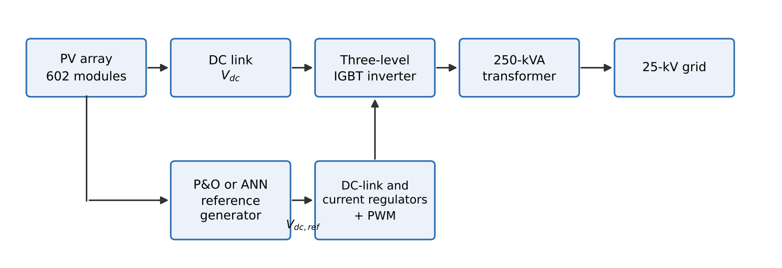
| Parameter | Value / status |
|---|---|
| PV module | SunPower SPR-415E-WHT-D |
| Module maximum power | 414.801 W |
| Open-circuit voltage, Voc | 85.3 V |
| Short-circuit current, Isc | approx. 6.09 A |
| MPP voltage, Vmp | 72.9 V |
| MPP current, Imp | 5.69 A |
| Cells per module | 128 |
| Series modules per string, Ns | 7 |
| Parallel strings, Np | 86 |
| Total module count | 602 |
| Calculated STC array rating | approx. 249.71 kW |
| Converter | Three-level IGBT bridge |
| Transformer | 250 kVA, 250 V/25 kV, three-phase |
| Grid frequency | 60 Hz |
| PWM carrier frequency | 1980 Hz in reference configuration |
2.2Array configuration and electrical model
The PV source used the SunPower SPR-415E-WHT-D monocrystalline module. The documented module values were approximately 414.801 W maximum power, 85.3 V open-circuit voltage, 6.09 A short-circuit current, 72.9 V voltage at maximum power, and 5.69 A current at maximum power [13]. The corrected array used seven modules in series per string and 86 parallel strings, giving
The nominal array power at standard test conditions (STC) is therefore
For interpretation, the PV source can be represented by the single-diode equation [14], [15]:
where Iph is the photo-generated current, I0 is diode saturation current, Rs and Rsh are series and shunt resistances, n is the diode ideality factor, Nc is the number of cells represented in series, and VT = kT/q is thermal voltage. The light-generated current varies approximately with irradiance:
These equations describe the physical basis of the PV block; the study retained the Simulink benchmark model rather than re-identifying every internal diode parameter.
3MPPT methods
3.1Perturb and observe
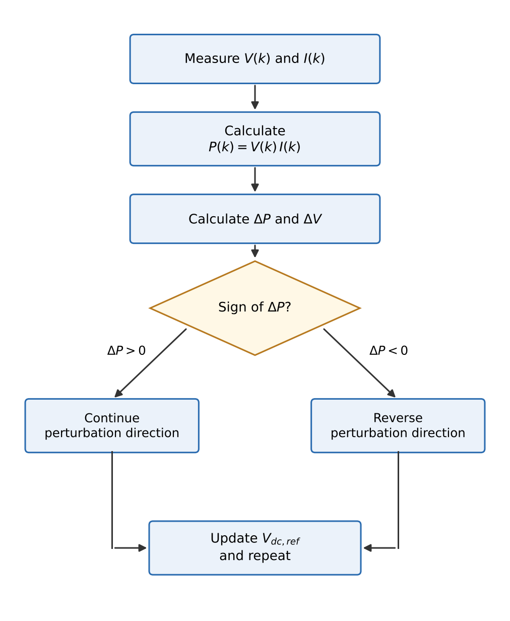
The retained P&O controller was implemented as a Stateflow state machine. At each update, measured PV voltage and current were used to calculate power. The controller compared successive samples:
The sign of ΔP, combined with the previous perturbation direction, determines whether the next voltage perturbation should continue or reverse (Figure 2). The generic reference update is
where s(k) ∈ {−1, +1}. If a perturbation increases power, the following perturbation continues in the same direction; if it decreases power, the direction reverses. The exact perturbation magnitude, Stateflow tolerances, initial reference, and sample time were not preserved in the written record and are not assumed here.
3.2Feedforward ANN reference generator
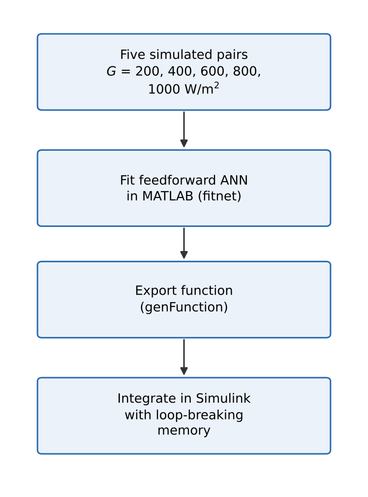
The ANN was implemented as a feedforward network with one hidden layer using MATLAB’s fitnet function; a generated MATLAB function was exported using genFunction and integrated into a copied Simulink model [16], [17]. The archived training set contained five simulation-generated operating pairs at irradiances of 200, 400, 600, 800, and 1000 W/m2, with corresponding reference voltages extracted from the P&O-controlled baseline. The recorded comparison held cell temperature at 45 °C. No physical PV measurements were used to construct this set. The development path is shown in Figure 3.
A generic one-hidden-layer mapping is
where xi are inputs, w and b are weights and biases, f is the hidden activation, and H is the hidden-neuron count. The fitting objective can be expressed as mean-squared error:
The hidden-neuron count and explicit training-algorithm settings were not preserved, so they are not reconstructed from software defaults. Memory block(s) were inserted to break an algebraic loop during Simulink integration. This means the ANN case was executable in the model, but the influence of that sample delay was not independently quantified.
4Simulation conditions and evaluation
The common environmental sequence began at 1000 W/m2, decreased to 200 W/m2, and was subsequently restored to 1000 W/m2. Cell temperature was held at 45 °C. The archived Scope displays covered approximately 1.5 s; exact disturbance transition timestamps were not preserved. Irradiance was assumed uniform across the array. Partial shading and hardware validation were outside the scope of the completed study.
| Quantity | Documented value / treatment |
|---|---|
| Initial irradiance | 1000 W/m2 |
| Reduced irradiance | 200 W/m2 |
| Final irradiance | 1000 W/m2 |
| Cell temperature | 45 °C (constant) |
| Recorded Scope duration | approximately 1.5 s |
| Irradiance distribution | Uniform |
| Grid frequency | 60 Hz |
| Hardware test | Not performed |
| ANN fitting points | 5 irradiance levels |
| Independent ANN test set | Not documented |
A rigorous comparison would require an independent MPP reference and synchronized numerical signals for both controllers. Common metrics include instantaneous tracking efficiency,
energy-based efficiency,
and power RMSE,
These metrics were not calculated because the independent reference trajectory and complete exported signal vectors were not retained. P&O output was not treated as ground truth for validating an ANN trained from that output.
5Results and discussion
5.1P&O reference operating points
At 1000 W/m2 and 45 °C, the documented operating point was approximately 481 V and 236 kW. At 200 W/m2, it was approximately 464 V and 46 kW. The irradiance change was
while the mean DC power change was
The DC-link voltage changed by
The large power change and comparatively small voltage shift are consistent with the fact that irradiance strongly affects photo-generated current, while the MPP voltage typically changes less at fixed temperature. When irradiance was restored, the archived Scope showed power and voltage returning toward the initial high-irradiance region. The screenshots did not preserve sufficient numerical data to calculate objective settling time, overshoot, or recovery time. The endpoint values are summarised in Table 3.
5.2ANN fitting and low-irradiance result
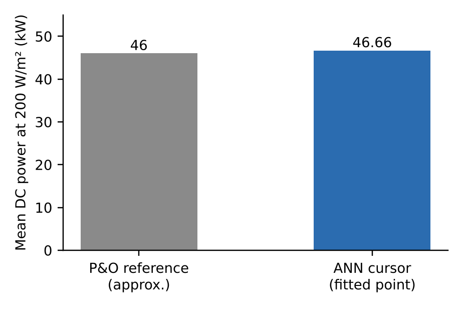
The ANN model was successfully integrated into the same plant architecture and exposed to the same high–low–high irradiance sequence. Its archived cursor measurement at 200 W/m2 recorded a mean DC power of 46.66 kW. Relative to the rounded 46-kW reference operating value, the absolute difference was 0.66 kW and the approximate relative endpoint difference was
This is an endpoint consistency check only. The 200-W/m2 condition was one of the five ANN fitting points, so it was not an unseen validation condition. In addition, the reference value is rounded and is not a full independent MPP time series. The two values are compared in Figure 4.
5.3What the comparison establishes
Table 4 separates documented outcomes from unavailable metrics. Both cases used the same plant and irradiance sequence, supporting a controlled qualitative comparison of endpoint behaviour. The ANN reproduced the low-irradiance operating region closely, but the record does not establish faster response, lower ripple, higher energy capture, better tracking efficiency, or lower computational cost.
| Item | Evidence | Interpretation |
|---|---|---|
| Plant and downstream control | Common architecture | Comparison structure controlled |
| Irradiance and temperature | 1000 → 200 → 1000 W/m2; 45 °C | Same disturbance sequence |
| P&O low-light power | approx. 46 kW | Reference operating region |
| ANN low-light power | 46.66 kW cursor | 1.43% endpoint difference from rounded value |
| Settling time | Not recovered numerically | No speed ranking |
| Steady-state ripple | Raw vectors unavailable | No ripple ranking |
| Energy efficiency | Independent MPP trajectory unavailable | No efficiency ranking |
| Unseen-condition generalization | No independent test set documented | Not established |
The ANN fitting set was very small and derived from the P&O-controlled model. Consequently, the ANN learned to reproduce a system-specific reference relationship rather than an independently measured physical MPP mapping. The ANN’s ability to generalize to unseen irradiance and temperature values remains unknown. This limitation is consistent with the wider MPPT literature, which emphasizes that tracking efficiency, transient response, oscillation, and validation conditions should be reported separately [2], [3], [9], [10].
6Limitations and recommendations
The principal limitations are: (1) only five simulation-derived points were used for ANN fitting; (2) the 200-W/m2 point was included in fitting; (3) the hidden-neuron count, explicit training settings, and some P&O parameters were not preserved in the written record; (4) the independent MPP trajectory and full numerical output vectors were unavailable; (5) no hardware or hardware-in-the-loop validation was performed; and (6) partial shading was not studied. The retained benchmark is a generic 60-Hz reference plant, not a location-specific grid model.
A repeat study should generate ANN targets from an independent PV model or a validated MPP calculation, use a wider irradiance–temperature grid, reserve genuinely unseen conditions for testing, and export synchronized irradiance, PV voltage, PV current, DC power, and reference-power signals. It should report MAE/RMSE, settling time under a declared tolerance, steady-state ripple, energy-based MPPT efficiency, and computational execution cost. The exact ANN architecture and P&O settings should be recorded, followed by hardware-in-the-loop or laboratory validation before claims about practical superiority are made.
7Conclusion
A feedforward ANN MPPT reference generator was integrated into a nominal 250-kW grid-connected PV benchmark and compared with the retained Stateflow P&O case under a common irradiance disturbance at 45 °C. The documented P&O operating points were approximately 481 V and 236 kW at 1000 W/m2, and 464 V and 46 kW at 200 W/m2. The ANN recorded 46.66 kW at the low-irradiance fitted point, approximately 1.43% above the rounded reference value. These findings support successful model integration and fitted-point reproduction. Because independent test data and numerical time-series signals were not available, no defensible conclusion can be made that ANN outperforms P&O in dynamics, energy efficiency, ripple, or computational cost. A stronger comparison requires independent MPP targets, broader training and test conditions, complete signal export, and reproducible controller parameters.
Acknowledgments
The author acknowledges the guidance and supervision of Samuel Pipelolu Olayiwola during the development of the thesis on which this paper is based.
References
- [1]International Energy Agency Photovoltaic Power Systems Programme. Trends in Photovoltaic Applications 2025. Report IEA PVPS T1-48:2025; 2025.
- [2]Boubaker O. MPPT techniques for photovoltaic systems: a systematic review in current trends and recent advances in artificial intelligence. Discover Energy. 2023;3:9. https://doi.org/10.1007/s43937-023-00024-2
- [3]Katche ML, Makokha AB, Zachary SO, Adaramola MS. A comprehensive review of maximum power point tracking (MPPT) techniques used in solar PV systems. Energies. 2023;16(5):2206. https://doi.org/10.3390/en16052206
- [4]Mazumdar D, Sain C, Biswas PK, Sanjeevikumar P, Khan B. Overview of solar photovoltaic MPPT methods: a state of the art on conventional and artificial intelligence control techniques. International Transactions on Electrical Energy Systems. 2024;2024:8363342. https://doi.org/10.1155/2024/8363342
- [5]Ahmed S, Mekhilef S, Mubin M, Tey KS, Kermadi K. An adaptive P&O algorithm with enhanced skipping feature for fast global maximum power point tracking under partial shading conditions. IEEE Transactions on Power Electronics. 2023;38(9):11601–11613. https://doi.org/10.1109/TPEL.2023.3285243
- [6]Harrison A, Nfah EM, Ndongmo JDDN, Alombah NH. An enhanced P&O MPPT algorithm for PV systems with fast dynamic and steady-state response under real irradiance and temperature conditions. International Journal of Photoenergy. 2022;2022:6009632. https://doi.org/10.1155/2022/6009632
- [7]Villegas-Mier CG, Rodriguez-Resendiz J, Alvarez-Alvarado JM, Rodriguez-Resendiz H, Herrera-Navarro AM, Rodriguez-Abreo O. Artificial neural networks in MPPT algorithms for optimization of photovoltaic power systems: a review. Micromachines. 2021;12(10):1260. https://doi.org/10.3390/mi12101260
- [8]Zecevic Z, Rolevski M. Neural network approach to MPPT control and irradiance estimation. Applied Sciences. 2020;10(15):5051. https://doi.org/10.3390/app10155051
- [9]Abouzeid AF, Eleraky H, Kalas A, Rizk R, Elsakka MM, Refaat A. Experimental validation of a low-cost maximum power point tracking technique based on artificial neural network for photovoltaic systems. Scientific Reports. 2024;14:18280. https://doi.org/10.1038/s41598-024-67306-0
- [10]Eyimaya SE. Efficiency analysis of artificial intelligence and conventional maximum power point tracking methods in photovoltaic systems. Applied Sciences. 2025;15(10):5586. https://doi.org/10.3390/app15105586
- [11]MathWorks. 250-kW grid-connected PV array. Simscape Electrical / Specialized Power Systems example documentation [Internet]. [cited 2026 Aug 25].
- [12]OPAL-RT Technologies. 250-kW grid-connected PV array. SPS software documentation [Internet]. Updated 2026 [cited 2026 Aug 25].
- [13]SunPower. SPR-415E-WHT-D photovoltaic module data, as documented in the adopted benchmark model.
- [14]Fahim SR, Hasanien HM, Turky RA, Abdel Aleem SHE, Calasan M. A comprehensive review of photovoltaic modules models and algorithms used in parameter extraction. Energies. 2022;15(23):8941. https://doi.org/10.3390/en15238941
- [15]Deotti LMP, da Silva Junior IC. A survey on the parameter extraction problem of the photovoltaic single diode model from a current–voltage curve. Solar Energy. 2023;263:111930. https://doi.org/10.1016/j.solener.2023.111930
- [16]MathWorks. fitnet: function fitting neural network. Deep Learning Toolbox documentation [Internet]. [cited 2026 Aug 25].
- [17]MathWorks. genFunction: generate MATLAB function for simulating shallow neural network. Deep Learning Toolbox documentation [Internet]. [cited 2026 Aug 25].