Comparative Analysis of Machine Learning Models for Diabetes Prediction

1Introduction

Diabetes mellitus is a chronic metabolic disease marked by high blood glucose. Late diagnosis often leads to complications affecting the heart, kidneys, eyes and nerves, so early screening is valuable. Machine learning (ML) can learn patterns from routine clinical measurements and support such screening [1].

Many ML algorithms have been applied to diabetes prediction, but their reported results depend on the data split, the handling of missing values and the tuning effort, which makes fair comparison difficult. This paper therefore evaluates eight common classifiers under identical conditions. The contributions are: (i) a controlled comparison of eight models using hold-out and repeated cross-validation, (ii) an analysis of hyperparameter tuning and class weighting, and (iii) confusion-matrix, ROC and feature-importance analysis.

2Related work

Smith et al. introduced the Pima Indians Diabetes data and used it to forecast the onset of diabetes with an early adaptive learning algorithm [2]. Since then it has become a standard benchmark. A survey of ML and data mining in diabetes research [1] notes that supervised learning is the most common approach, with methods such as support vector machines, decision trees and ensembles widely used for prediction and diagnosis.

However, published results on this dataset are not always comparable, because studies differ in preprocessing, missing-value handling and evaluation method. This work uses one fixed pipeline for all models and reports both single-split and repeated cross-validation results.

3Dataset and preprocessing

3.1Dataset

The Pima Indians Diabetes dataset [2] contains 768 female patients aged 21 years or older, of whom 268 (34.9%) are diabetic and 500 (65.1%) are not. The eight features are the number of pregnancies, plasma glucose, diastolic blood pressure, skin-fold thickness, insulin, body mass index (BMI), diabetes pedigree function and age. The target is a binary outcome (diabetic or not). Table 1 summarizes the features.

Feature	Mean	SD	Min	Max	Zeros
Pregnancies	3.85	3.37	0	17	0
Glucose	121.69	30.54	44	199	5
Blood pressure	72.41	12.38	24	122	35
Skin thickness	29.15	10.48	7	99	227
Insulin	155.55	118.78	14	846	374
BMI	32.46	6.92	18.2	67.1	11
Pedigree func.	0.47	0.33	0.08	2.42	0
Age	33.24	11.76	21	81	0

3.2Preprocessing

In glucose, blood pressure, skin thickness, insulin and BMI, a value of zero is physiologically impossible and indicates a missing entry. The number of such zeros is given in Table 1; insulin (48.7%) and skin thickness (29.6%) are the most affected. These zeros were converted to missing values and imputed with the column median. Features were then standardized to zero mean and unit variance. The data were split 80/20 with stratification (random seed 42), giving 614 training and 154 test records. Imputation and scaling were fitted inside a pipeline on training data only, to avoid data leakage.

4Methodology

4.1Models

Eight classifiers were implemented with scikit-learn [3]. Logistic Regression (LR) [4] models the probability of diabetes with a linear decision boundary. k-Nearest Neighbors (KNN) [5] labels a patient by the majority class among the nearest training records. The Support Vector Machine (SVM) [6] with an RBF kernel finds a maximum-margin boundary in a transformed space. Gaussian Naive Bayes (NB) [7] applies Bayes’ rule assuming independent features. The Decision Tree (DT) [8] splits the data with simple if-then rules. Random Forest (RF) [9] averages many decorrelated trees. AdaBoost [10] combines weak learners by re-weighting misclassified samples, and Gradient Boosting (GB) [11] adds trees that correct the errors of the previous ones.

4.2Experimental setup

Four experiments were run. First, baseline models with common settings (KNN with k = 7, DT with depth 5, RF with 300 trees, AdaBoost with 200 estimators, others default) were trained on the training set and evaluated on the test set. Second, to reduce dependence on one split, each baseline model was evaluated on the full dataset with stratified 10-fold cross-validation repeated three times (30 folds). Third, hyperparameters were tuned by grid search with 5-fold cross-validation on the training set, selecting the setting with the best ROC-AUC. Fourth, class weighting was applied to four models to study its effect on recall.

4.3Evaluation metrics

Diabetic cases are the positive class. With true positives (TP), true negatives (TN), false positives (FP) and false negatives (FN), the metrics are:

The area under the ROC curve (ROC-AUC) [12] measures how well a model ranks diabetic patients above non-diabetic ones across all thresholds. Recall is especially important in screening, because a false negative is a missed patient.

5Results

5.1Baseline hold-out results

Table 2 shows the baseline results on the 154 test records. The best value in each column is in bold.

Model	Accuracy	Precision	Recall	F1	ROC-AUC
Logistic Regression	0.708	0.600	0.500	0.545	0.813
KNN	0.727	0.625	0.556	0.588	0.790
SVM (RBF)	0.740	0.652	0.556	0.600	0.796
Naive Bayes	0.701	0.567	0.630	0.596	0.765
Decision Tree	0.760	0.639	0.722	0.678	0.762
Random Forest	0.740	0.659	0.537	0.592	0.816
AdaBoost	0.760	0.681	0.593	0.634	0.818
Gradient Boosting	0.760	0.689	0.574	0.626	0.831

Decision Tree, AdaBoost and Gradient Boosting tied for the highest accuracy (76.0%). Gradient Boosting gave the best ROC-AUC (0.831) and precision (0.689), while the Decision Tree gave the best recall (0.722) and F1-score (0.678).

5.2Repeated cross-validation

Table 3 reports the mean and standard deviation over 30 folds. This estimate is more reliable than a single split of 154 records.

Model	Accuracy	F1-score	ROC-AUC
Logistic Regression	0.766 ± 0.042	0.618 ± 0.081	0.837 ± 0.048
KNN	0.746 ± 0.052	0.618 ± 0.087	0.807 ± 0.052
SVM (RBF)	0.754 ± 0.044	0.600 ± 0.084	0.831 ± 0.043
Naive Bayes	0.746 ± 0.047	0.617 ± 0.077	0.816 ± 0.046
Decision Tree	0.745 ± 0.048	0.628 ± 0.081	0.784 ± 0.065
Random Forest	0.764 ± 0.043	0.643 ± 0.075	0.832 ± 0.052
AdaBoost	0.757 ± 0.046	0.626 ± 0.074	0.828 ± 0.048
Gradient Boosting	0.769 ± 0.046	0.649 ± 0.079	0.833 ± 0.051

Gradient Boosting had the highest mean accuracy (0.769) and F1-score (0.649), closely followed by Logistic Regression (0.766) and Random Forest (0.764). Logistic Regression had the highest ROC-AUC (0.837). The Decision Tree had the lowest ROC-AUC (0.784), which shows that its good hold-out recall was partly due to the particular split. Standard deviations of about 0.04–0.05 are larger than the gaps between the top models, so these models are practically equivalent on this dataset.

5.3Hyperparameter tuning

Table 4 gives the test results of the tuned models.

Model	Accuracy	Precision	Recall	F1	ROC-AUC
Logistic Regression	0.688	0.565	0.481	0.520	0.810
KNN	0.734	0.644	0.537	0.586	0.807
SVM (RBF)	0.708	0.610	0.463	0.526	0.805
Naive Bayes	0.701	0.567	0.630	0.596	0.765
Decision Tree	0.786	0.698	0.685	0.692	0.789
Random Forest	0.727	0.636	0.519	0.571	0.813
AdaBoost	0.734	0.651	0.519	0.577	0.818
Gradient Boosting	0.721	0.622	0.519	0.566	0.815

Tuning (e.g., k = 15 for KNN, depth 4 for the Decision Tree) did not improve every model. Accuracy rose for KNN (0.727 to 0.734) and for the Decision Tree (0.760 to 0.786), which became the best tuned model on accuracy, precision, recall and F1-score. For Logistic Regression, SVM, Random Forest, AdaBoost and Gradient Boosting, test accuracy fell by 1.3 to 3.9 points. Since the grid search optimized ROC-AUC on the training folds and the test set is small, these changes mainly show the variability of a single split rather than a real loss.

5.4ROC and error analysis

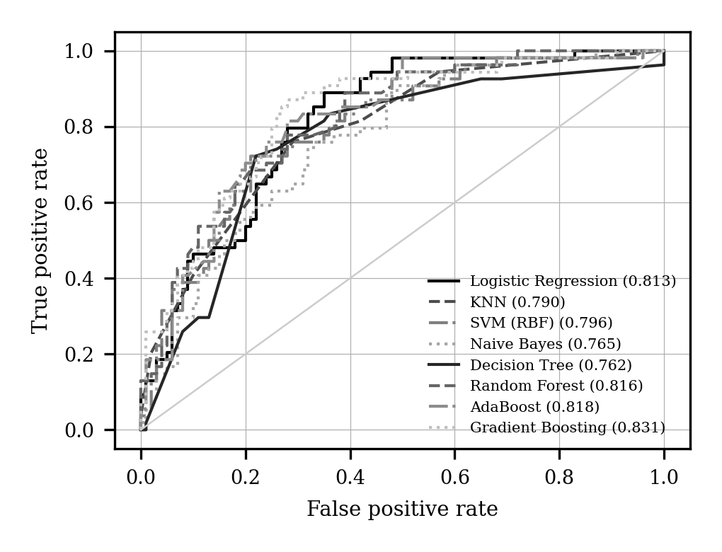
Figure 1 shows that the ensemble models and Logistic Regression lie close together, above the Decision Tree and Naive Bayes curves, as the AUC values in Table 2 indicate. On the test set (100 non-diabetic and 54 diabetic patients), the Decision Tree missed 15 diabetic patients (27.8%) and Naive Bayes missed 20, whereas Logistic Regression missed 27 (50.0%). The cost of fewer misses was more false alarms: the Decision Tree and Naive Bayes produced 22 and 26 false positives, compared with 14 for Gradient Boosting.

5.5Effect of class weighting

Because only 34.9% of patients are diabetic, models tend to favor the majority class. Table 5 shows the effect of balanced class weights.

Model	Accuracy	Precision	Recall	F1	ROC-AUC
Logistic Regression	0.734	0.603	0.704	0.650	0.813
SVM (RBF)	0.727	0.591	0.722	0.650	0.814
Decision Tree	0.727	0.611	0.611	0.611	0.771
Random Forest	0.734	0.644	0.537	0.586	0.816

Class weighting raised the recall of Logistic Regression from 0.500 to 0.704 and of SVM from 0.556 to 0.722, and their F1-scores rose from 0.545 to 0.650 and from 0.600 to 0.650. It did not help the Decision Tree (F1 fell from 0.678 to 0.611) or Random Forest (recall stayed at 0.537). Thus class weighting is a simple and effective choice for linear and kernel models, but not for every model.

5.6Feature importance

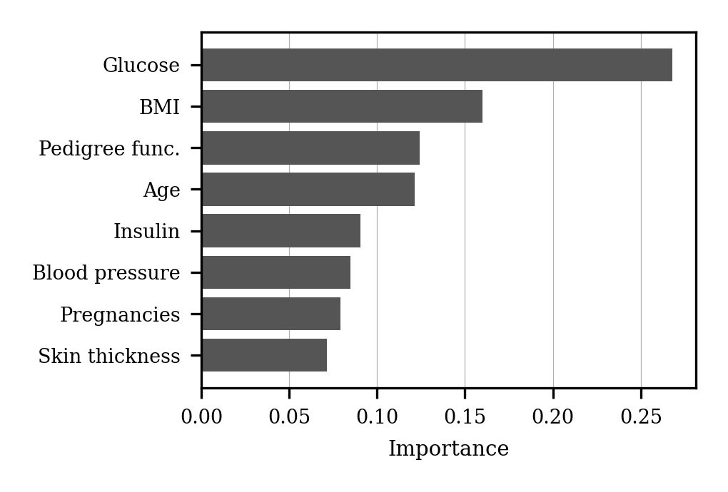
Figure 2 shows that glucose was the most important feature (0.268), followed by BMI (0.160), diabetes pedigree function (0.124) and age (0.121). This agrees with clinical knowledge that blood glucose and body weight are key risk indicators.

6Discussion

Three observations stand out. First, no model was best on every metric, and rankings changed between the hold-out split and repeated cross-validation. Gradient Boosting, Random Forest and Logistic Regression were consistently among the top models, while the Decision Tree looked strong on one split but was the weakest in ROC-AUC under cross-validation.

Second, a simple model such as Logistic Regression performed as well as complex ensembles, which is plausible with only 768 records and 8 features.

Third, the choice of model should depend on the goal. For screening, where missing a patient is costly, a model with higher recall, or a class-weighted Logistic Regression or SVM, may be preferred even at the cost of more false alarms.

Limitations. The dataset is small and contains only women of Pima heritage aged 21 or older, so the results may not generalize to other populations. Many insulin and skin-thickness values were missing and had to be imputed. Hyperparameter grids were small, and no external validation was done.

7Conclusion

This paper compared eight ML classifiers for diabetes prediction under one preprocessing pipeline using hold-out testing, repeated cross-validation, tuning and class weighting. Gradient Boosting had the highest cross-validated accuracy (76.9%) and F1-score, Logistic Regression had the highest ROC-AUC (0.837), and the top models differed by less than one standard deviation. Class weighting substantially improved recall for Logistic Regression and SVM, and glucose was the strongest predictor. Future work will explore larger and more diverse datasets, better missing-value handling, probability calibration, and external validation.

References

1. [1]Kavakiotis I, Tsave O, Salifoglou A, Maglaveras N, Vlahavas I, Chouvarda I. Machine learning and data mining methods in diabetes research. Computational and Structural Biotechnology Journal. 2017;15:104–116.
2. [2]Smith JW, Everhart JE, Dickson WC, Knowler WC, Johannes RS. Using the ADAP learning algorithm to forecast the onset of diabetes mellitus. In: Proceedings of the Annual Symposium on Computer Application in Medical Care; 1988. p. 261–265.
3. [3]Pedregosa F, Varoquaux G, Gramfort A, Michel V, Thirion B, Grisel O, et al. Scikit-learn: Machine learning in Python. Journal of Machine Learning Research. 2011;12:2825–2830.
4. [4]Cox DR. The regression analysis of binary sequences. Journal of the Royal Statistical Society: Series B. 1958;20(2):215–242.
5. [5]Cover T, Hart P. Nearest neighbor pattern classification. IEEE Transactions on Information Theory. 1967;13(1):21–27.
6. [6]Cortes C, Vapnik V. Support-vector networks. Machine Learning. 1995;20(3):273–297.
7. [7]Hastie T, Tibshirani R, Friedman J. The elements of statistical learning. 2nd ed. New York (NY): Springer; 2009.
8. [8]Quinlan JR. Induction of decision trees. Machine Learning. 1986;1(1):81–106.
9. [9]Breiman L. Random forests. Machine Learning. 2001;45(1):5–32.
10. [10]Freund Y, Schapire RE. A decision-theoretic generalization of on-line learning and an application to boosting. Journal of Computer and System Sciences. 1997;55(1):119–139.
11. [11]Friedman JH. Greedy function approximation: A gradient boosting machine. Annals of Statistics. 2001;29(5):1189–1232.
12. [12]Fawcett T. An introduction to ROC analysis. Pattern Recognition Letters. 2006;27(8):861–874.